<?xml version="1.0" encoding="utf-8"?><feed xmlns="http://www.w3.org/2005/Atom" ><generator uri="https://jekyllrb.com/" version="4.3.2">Jekyll</generator><link href="/preview/pr-10/feed.xml" rel="self" type="application/atom+xml" /><link href="/preview/pr-10/" rel="alternate" type="text/html" /><updated>2026-10-10T14:59:13+00:00</updated><id>/preview/pr-10/feed.xml</id><title type="html">Agentic Intelligence Lab</title><subtitle>Our team at the Department of Data and Systems Engineering, The University of Hong Kong, is dedicated to advancing research in Machine Learning, Sequential Decision Making, and Embodied AI.</subtitle><entry><title type="html">RL4F — Offline Reinforcement Learning for Plasma Control in Nuclear Fusion</title><link href="/preview/pr-10/2026/10/10/rl4f-post.html" rel="alternate" type="text/html" title="RL4F — Offline Reinforcement Learning for Plasma Control in Nuclear Fusion" /><published>2026-10-10T00:00:00+00:00</published><updated>2026-10-10T14:58:01+00:00</updated><id>/preview/pr-10/2026/10/10/rl4f-post</id><content type="html" xml:base="/preview/pr-10/2026/10/10/rl4f-post.html"><![CDATA[<!-- excerpt start -->
<p><strong>RL4F</strong> is an open-source benchmark for learning plasma controllers from offline data. Built around a dynamics ensemble trained on historical DIII-D tokamak discharges, it provides datasets, closed-loop evaluation environments, and baselines for rotation, density, electron temperature, and pressure profile tracking.
<!-- excerpt end --></p>

<p>Our paper, <strong>“Offline Reinforcement Learning for Plasma Control in Nuclear Fusion: Codebase and Benchmark,”</strong> introduces a common testbed for comparing offline RL algorithms on a demanding physical control problem.</p>

<p>Yang Fu*, Haomin Bao*, Rohit Sonker, Xiaoyan Hu, Aravind Venugopal, Jeff Schneider, Jiayu Chen</p>

<p><sub>*Equal contribution</sub></p>

<p><a href="https://arxiv.org/abs/2606.07550">Paper</a> · <a href="https://yywoai66.github.io/RL4F/">Project page</a> · <a href="https://github.com/LucasCJYSDL/Offline-RL-Kit-for-Nuclear-Fusion">Code</a> · <a href="https://huggingface.co/datasets/Neurips-ED-submission-685/fusion-rl-benchmark">Dataset</a> · <a href="https://huggingface.co/Neurips-ED-submission-685/fusion-rl-dynamics-model">Dynamics models</a></p>

<h2 id="why-plasma-control-needs-an-offline-benchmark">Why plasma control needs an offline benchmark</h2>

<p>A tokamak controller must regulate a plasma whose behavior is nonlinear, coupled, and sensitive to its operating conditions. Changing heating, torque, or fueling affects several quantities at once, and the response unfolds over time.</p>

<p>The goal is also spatial: a plasma <em>profile</em> describes how a quantity varies from the core to the edge. Holding one scalar near its target does not necessarily produce the desired profile throughout the plasma.</p>

<p>Developing a controller through trial and error on a real device is expensive and risky. Historical experiments offer a starting point, but algorithm development also needs shared datasets and evaluation conditions. RL4F supplies that common ground, so researchers can compare how their methods handle the same tracking tasks before considering real-machine experiments.</p>

<h2 id="from-experimental-discharges-to-policy-evaluation">From experimental discharges to policy evaluation</h2>

<figure class="figure">
  <a class="figure-image" aria-label="The RL4F reference dynamics ensemble connects historical DIII-D discharges to a closed-loop policy evaluation environment. Figure from the RL4F project.">
    <img src="/preview/pr-10/images/RL4F/benchmark-rpnn-workflow.png" style="
        width: 100%;
        max-height: unset;
      " alt="The RL4F reference dynamics ensemble connects historical DIII-D discharges to a closed-loop policy evaluation environment. Figure from the RL4F project." loading="lazy" onerror="this.src = '/preview/pr-10/images/fallback.svg'; this.onerror = null;" />
  </a>
  
    <figcaption class="figure-caption">
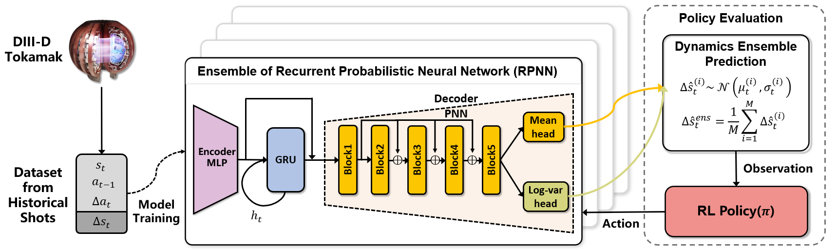
      The RL4F reference dynamics ensemble connects historical DIII-D discharges to a closed-loop policy evaluation environment. Figure from the RL4F project.

    </figcaption>
  
</figure>

<p>RL4F starts with a <strong>25-member ensemble of recurrent probabilistic neural networks (RPNNs)</strong> trained on roughly <strong>18,000 historical DIII-D discharges</strong>, with measurements sampled every <strong>20 ms</strong>. Each model predicts a distribution over the next plasma-state change from the current state and actuator inputs.</p>

<p>Training proceeds in two stages: first learn the predictive mean, then freeze the mean-prediction backbone and fit the variance head. The ensemble represents different plausible dynamics, while the variance head models uncertainty in each member’s predictions.</p>

<p>The released offline RL trajectories are <strong>model-generated</strong>. We initialize the reference model from experimental shot states, replay the recorded actuator schedules, and roll the model forward. This preserves the experimental action sequences while replacing the measured plasma evolution with simulated trajectories.</p>

<p>After filtering, the dataset contains <strong>5,882 shots and 945,828 transitions</strong>, with fixed splits:</p>

<table>
  <thead>
    <tr>
      <th>Split</th>
      <th style="text-align: right">Shots</th>
      <th style="text-align: right">Transitions</th>
    </tr>
  </thead>
  <tbody>
    <tr>
      <td>Training</td>
      <td style="text-align: right">5,282</td>
      <td style="text-align: right">849,977</td>
    </tr>
    <tr>
      <td>Validation</td>
      <td style="text-align: right">300</td>
      <td style="text-align: right">48,010</td>
    </tr>
    <tr>
      <td>Test</td>
      <td style="text-align: right">300</td>
      <td style="text-align: right">47,841</td>
    </tr>
  </tbody>
</table>

<p>Model-based baselines fit their own dynamics models from these synthetic training trajectories. Trained policies are then evaluated in closed loop against the reference ensemble, separating the models used for policy learning from the benchmark environment.</p>

<h2 id="four-tasks-one-shared-actuator-space">Four tasks, one shared actuator space</h2>

<p>The paper studies four full-profile tracking objectives:</p>

<table>
  <thead>
    <tr>
      <th>Tracking target</th>
      <th>Task flag</th>
      <th>Control objective</th>
    </tr>
  </thead>
  <tbody>
    <tr>
      <td>Rotation</td>
      <td><code class="language-plaintext highlighter-rouge">rotation</code></td>
      <td>Track the radial rotation profile</td>
    </tr>
    <tr>
      <td>Electron density</td>
      <td><code class="language-plaintext highlighter-rouge">dens</code></td>
      <td>Track the radial density profile</td>
    </tr>
    <tr>
      <td>Electron temperature</td>
      <td><code class="language-plaintext highlighter-rouge">temp</code></td>
      <td>Track the radial electron-temperature profile</td>
    </tr>
    <tr>
      <td>Pressure</td>
      <td><code class="language-plaintext highlighter-rouge">pres</code></td>
      <td>Track the radial pressure profile</td>
    </tr>
  </tbody>
</table>

<p>Every task uses the same four actuation channels: <strong>neutral-beam power, neutral-beam torque, gas puffing, and electron-cyclotron heating power</strong>. The policy receives the current profile, current and future targets, and explicit tracking-error terms.</p>

<p>Targets change during each rollout, requiring the controller to respond to a new setpoint and maintain it over time. Tracking is measured across <strong>33 radial locations</strong>, rather than judged only from a scalar summary.</p>

<h2 id="what-the-benchmark-reveals">What the benchmark reveals</h2>

<p>We compare goal-conditioned imitation learning, model-free offline RL methods such as TD3BC, CQL, IQL, EDAC, and MCQ, and model-based methods including PPO, COMBO, MOPO, MOBILE, RAMBO, and BAMCTS.</p>

<p>Evaluation uses <strong>300 held-out test shots with 10 random seeds per shot</strong>. The <a href="https://arxiv.org/html/2606.07550v1#S5">paper’s main results</a> report the following best task-average tracking errors:</p>

<table>
  <thead>
    <tr>
      <th>Task</th>
      <th>Best method</th>
      <th style="text-align: right">Average RMSE ± standard error</th>
    </tr>
  </thead>
  <tbody>
    <tr>
      <td>Rotation</td>
      <td>RAMBO</td>
      <td style="text-align: right">8.03 ± 0.029</td>
    </tr>
    <tr>
      <td>Density</td>
      <td>COMBO</td>
      <td style="text-align: right">0.691 ± 0.0017</td>
    </tr>
    <tr>
      <td>Electron temperature</td>
      <td>MOPO</td>
      <td style="text-align: right">0.193 ± 0.0005</td>
    </tr>
    <tr>
      <td>Pressure</td>
      <td>MOPO</td>
      <td style="text-align: right">5,198.6 ± 16.5</td>
    </tr>
  </tbody>
</table>

<p><em>Lower is better. Each task has its own physical scale; these raw RMSE values should be compared within a task.</em></p>

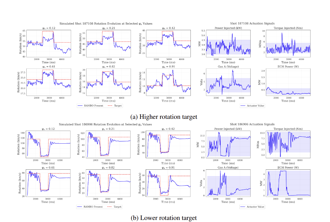
<p>The strongest method changes with the control objective. RAMBO performs well on rotation but struggles on density and temperature. COMBO leads density tracking, while MOPO achieves the lowest average error on temperature and pressure. Model-based approaches obtain the best averages across these tasks, but using a learned model alone does not guarantee strong performance.</p>

<figure class="figure">
  <a class="figure-image" aria-label="RAMBO rotation-control rollouts in the learned dynamics environment. Profile traces on the left show the response to higher and lower targets; actuator traces on the right show the coordinated control actions. These are simulated evaluations. Figure from the RL4F project.">
    <img src="/preview/pr-10/images/RL4F/rotation-tracking.png" style="
        width: 100%;
        max-height: unset;
      " alt="RAMBO rotation-control rollouts in the learned dynamics environment. Profile traces on the left show the response to higher and lower targets; actuator traces on the right show the coordinated control actions. These are simulated evaluations. Figure from the RL4F project." loading="lazy" onerror="this.src = '/preview/pr-10/images/fallback.svg'; this.onerror = null;" />
  </a>
  
    <figcaption class="figure-caption">
      RAMBO rotation-control rollouts in the learned dynamics environment. Profile traces on the left show the response to higher and lower targets; actuator traces on the right show the coordinated control actions. These are simulated evaluations. Figure from the RL4F project.

    </figcaption>
  
</figure>

<h2 id="try-rl4f">Try RL4F</h2>

<p>The repository provides environment setup instructions, pre-trained dynamics models, algorithm entry points, and a unified visualization script.</p>

<ol>
  <li>Follow the <a href="https://github.com/LucasCJYSDL/Offline-RL-Kit-for-Nuclear-Fusion#quick-start">README’s Quick Start</a> to install the Conda environment and dependencies.</li>
  <li>Download the <a href="https://huggingface.co/datasets/Neurips-ED-submission-685/fusion-rl-benchmark/tree/main/processed">processed datasets</a> and <a href="https://huggingface.co/Neurips-ED-submission-685/fusion-rl-dynamics-model">dynamics models</a>, then place them in the directories described in the README.</li>
  <li>Run a temperature-control baseline from the source checkout:</li>
</ol>

<div class="language-bash highlighter-rouge"><div class="highlight"><pre class="highlight"><code>python scripts/run_ppo.py <span class="nt">--env</span> profile_control_new <span class="nt">--task</span> temp
</code></pre></div></div>

<p>Training scripts load the matching task and algorithm defaults from <code class="language-plaintext highlighter-rouge">offlinerlkit/configs/benchmark_configs.json</code>. Command-line arguments override these defaults, and policy checkpoints and return plots are saved under <code class="language-plaintext highlighter-rouge">logs/</code>.</p>

<p>To inspect a trained policy, replace <code class="language-plaintext highlighter-rouge">/path/to/your_run_dir</code> with its run directory:</p>

<div class="language-bash highlighter-rouge"><div class="highlight"><pre class="highlight"><code>python <span class="nt">-m</span> visualization.profile_tracking_save <span class="nt">--actor_path</span> /path/to/your_run_dir <span class="nt">--test</span>
</code></pre></div></div>

<p>The script saves actuator trajectories, profile-tracking outputs, and tracking-error summaries under <code class="language-plaintext highlighter-rouge">results/&lt;task&gt;/&lt;algo&gt;/&lt;val|test&gt;/&lt;run&gt;/&lt;seed&gt;/</code>.</p>

<h2 id="what-remains-open">What remains open</h2>

<p>RL4F measures control performance in a learned environment derived from DIII-D data. Its results do not establish how these policies will behave on a real tokamak or transfer to another device. Model error and the simulation-to-reality gap remain important questions for future experiments.</p>

<p>By releasing the datasets, reference models, code, and evaluation protocol, we aim to make those questions easier to study and give offline RL researchers a reproducible setting for developing better plasma controllers.</p>

<h2 id="citation">Citation</h2>

<div class="language-bibtex highlighter-rouge"><div class="highlight"><pre class="highlight"><code><span class="nc">@misc</span><span class="p">{</span><span class="nl">fu2026offline</span><span class="p">,</span>
  <span class="na">title</span><span class="p">=</span><span class="s">{Offline Reinforcement Learning for Plasma Control in Nuclear Fusion: Codebase and Benchmark}</span><span class="p">,</span>
  <span class="na">author</span><span class="p">=</span><span class="s">{Yang Fu and Haomin Bao and Rohit Sonker and Xiaoyan Hu and Aravind Venugopal and Jeff Schneider and Jiayu Chen}</span><span class="p">,</span>
  <span class="na">year</span><span class="p">=</span><span class="s">{2026}</span><span class="p">,</span>
  <span class="na">eprint</span><span class="p">=</span><span class="s">{2606.07550}</span><span class="p">,</span>
  <span class="na">archivePrefix</span><span class="p">=</span><span class="s">{arXiv}</span><span class="p">,</span>
  <span class="na">primaryClass</span><span class="p">=</span><span class="s">{cs.LG}</span><span class="p">,</span>
  <span class="na">url</span><span class="p">=</span><span class="s">{https://arxiv.org/abs/2606.07550}</span>
<span class="p">}</span>
</code></pre></div></div>]]></content><author><name>Yang Fu</name></author><category term="publication" /><category term="offline-rl" /><category term="nuclear-fusion" /><category term="plasma-control" /><category term="benchmark" /><summary type="html"><![CDATA[RL4F is an open-source benchmark for learning plasma controllers from offline data. Built around a dynamics ensemble trained on historical DIII-D tokamak discharges, it provides datasets, closed-loop evaluation environments, and baselines for rotation, density, electron temperature, and pressure profile tracking.]]></summary><media:thumbnail xmlns:media="http://search.yahoo.com/mrss/" url="/preview/pr-10/images/RL4F/benchmark-rpnn-workflow.png" /><media:content medium="image" url="/preview/pr-10/images/RL4F/benchmark-rpnn-workflow.png" xmlns:media="http://search.yahoo.com/mrss/" /></entry><entry><title type="html">CausalVAE as a Plug-in for World Models: Towards Reliable Counterfactual Dynamics (ECCV 2026)</title><link href="/preview/pr-10/2026/08/10/causalvae-world-models.html" rel="alternate" type="text/html" title="CausalVAE as a Plug-in for World Models: Towards Reliable Counterfactual Dynamics (ECCV 2026)" /><published>2026-08-10T00:00:00+00:00</published><updated>2026-10-10T14:58:01+00:00</updated><id>/preview/pr-10/2026/08/10/causalvae-world-models</id><content type="html" xml:base="/preview/pr-10/2026/08/10/causalvae-world-models.html"><![CDATA[<h3 id="predicting-is-not-yet-understanding">Predicting Is Not Yet Understanding</h3>

<p><em>ECCV 2026 · Causal World Models</em></p>

<p>Ziyi Ding, Xianxin Lai, Weiyu Chen, Xiao-Ping Zhang, Jiayu Chen</p>

<p>Tsinghua Shenzhen International Graduate School · The University of Hong Kong · INFIFORCE Intelligent Technology</p>

<div class="button-wrapper">
    <a class="button" href="https://arxiv.org/pdf/2604.07712" data-tooltip="Paper" data-style="" aria-label="Paper">
      <i class="icon fa-solid fa-scroll"></i>
      
        <span>Read the paper</span>
      
    </a>
  </div>

<figure class="figure">
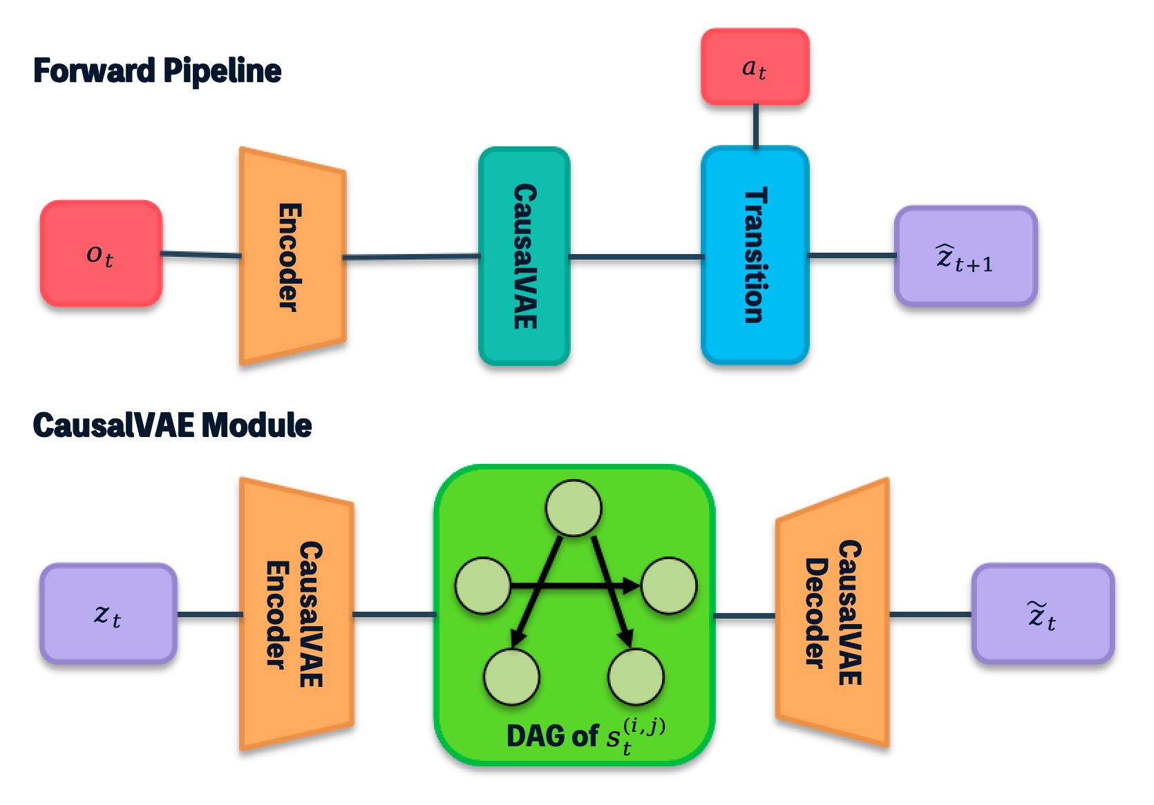
  <a class="figure-image" aria-label="The forward pipeline inserts CausalVAE between the encoder and action-conditioned transition. The module maps the backbone latent through an encoder, a learned directed acyclic graph DAG , and a decoder.">
    <img src="/preview/pr-10/images/CausalVAE/method-overview.png" style="
        width: 100%;
        max-height: unset;
      " alt="The forward pipeline inserts CausalVAE between the encoder and action-conditioned transition. The module maps the backbone latent through an encoder, a learned directed acyclic graph DAG , and a decoder." loading="lazy" onerror="this.src = '/preview/pr-10/images/fallback.svg'; this.onerror = null;" />
  </a>
  
    <figcaption class="figure-caption">
      The forward pipeline inserts CausalVAE between the encoder and action-conditioned transition. The module maps the backbone latent through an encoder, a learned directed acyclic graph (DAG), and a decoder.

    </figcaption>
  
</figure>

<p>A world model should not only say what happens next. It should also know what would happen if something changed.</p>

<p>Latent world models compress images into compact states and roll them forward under actions. That recipe works well for factual prediction: given what actually happened, retrieve or generate the most likely future. But the same latent can be unreliable under an intervention, because features that are useful for prediction are not necessarily separated into causes and effects.</p>

<p>A counterfactual query is more demanding. If we move one object, change its velocity, or alter a mechanism, the model must update the variables downstream of that change while leaving unrelated factors alone. In an entangled latent space, the intervention often becomes a diffuse perturbation: too much changes, too little changes, or the effect travels along the wrong path.</p>

<p>Our question is simple: <strong>can we add explicit causal structure to an existing world model without redesigning the predictive backbone?</strong></p>

<h2 id="attach-causal-structure-where-the-world-model-already-reasons">Attach causal structure where the world model already reasons</h2>

<p>We introduce a CausalVAE-inspired structural branch directly in latent space. The original encoder still maps an observation to a latent state, and the original action-conditioned transition still predicts the next latent. Between them, our plug-in organizes latent factors through a learned DAG:</p>

<div class="alert" style="--color: #0ea5e9">
  
  <i class="icon fa-solid fa-circle-info"></i>
  <div class="alert-content">
    <p><strong>Plug-in design:</strong> observation <em>oₜ</em> → encoder <em>E</em> → latent <em>zₜ</em> → CausalVAE → transition <em>F</em> → future <em>ẑₜ₊₁</em>.</p>

  </div>
</div>

<p>The key is modularity. The same structural branch can sit on AE, VAE, modular, or graph-network dynamics backbones. A differentiable acyclicity penalty keeps the learned adjacency close to a DAG, while a lightweight alignment head anchors latent coordinates to simulator state during training. Neither simulator state nor the alignment head is needed at inference.</p>

<h2 id="a-three-stage-training-strategy">A three-stage training strategy</h2>

<figure class="figure">
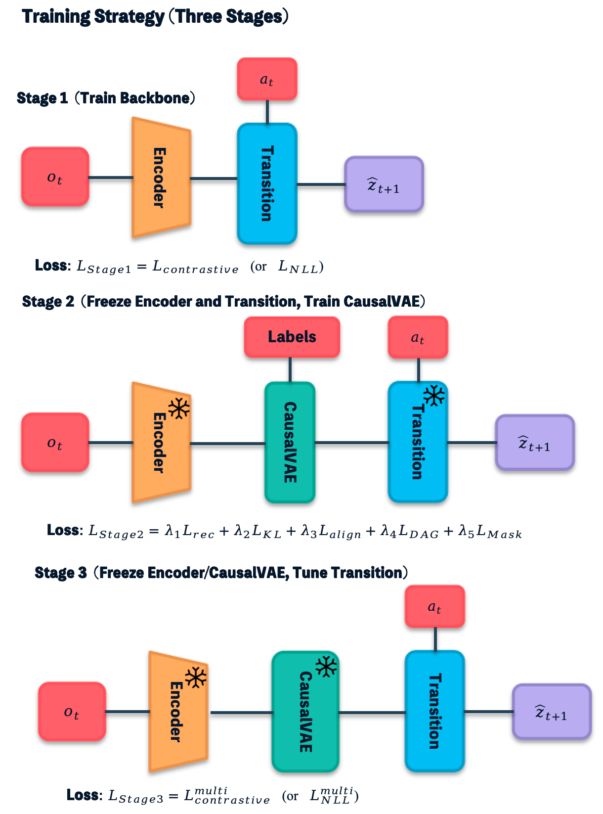
  <a class="figure-image" aria-label="Stage 1 trains the predictive backbone. Stage 2 freezes the encoder and transition while fitting the structural branch. Stage 3 freezes the encoder and CausalVAE while tuning the transition on multi-step objectives.">
    <img src="/preview/pr-10/images/CausalVAE/training-strategy.png" style="
        width: min(100%, 720px);
        max-height: unset;
      " alt="Stage 1 trains the predictive backbone. Stage 2 freezes the encoder and transition while fitting the structural branch. Stage 3 freezes the encoder and CausalVAE while tuning the transition on multi-step objectives." loading="lazy" onerror="this.src = '/preview/pr-10/images/fallback.svg'; this.onerror = null;" />
  </a>
  
    <figcaption class="figure-caption">
      Stage 1 trains the predictive backbone. Stage 2 freezes the encoder and transition while fitting the structural branch. Stage 3 freezes the encoder and CausalVAE while tuning the transition on multi-step objectives.

    </figcaption>
  
</figure>

<div class="cols" style="--cols: 3">
  
    
    <div>
<h3 id="01--predict">01 · Predict</h3>

<p>Train the encoder and transition backbone on standard world-model objectives.</p>
</div>
  
    
    <div>
<h3 id="02--structure">02 · Structure</h3>

<p>Freeze the backbone and learn the causal branch with reconstruction, KL, alignment, and DAG constraints.</p>
</div>
  
    
    <div>
<h3 id="03--refine">03 · Refine</h3>

<p>Freeze the encoder and CausalVAE, then tune the transition with an α-gated mixture and multi-step supervision.</p>
</div>
  
</div>

<p>This staged design lets the backbone first acquire predictive competence, gives the structural branch a stable representation to organize, and finally adapts the transition to the causally structured latent without retraining the entire system from scratch.</p>

<h2 id="intervene-re-simulate-then-retrieve-the-right-future">Intervene, re-simulate, then retrieve the right future</h2>

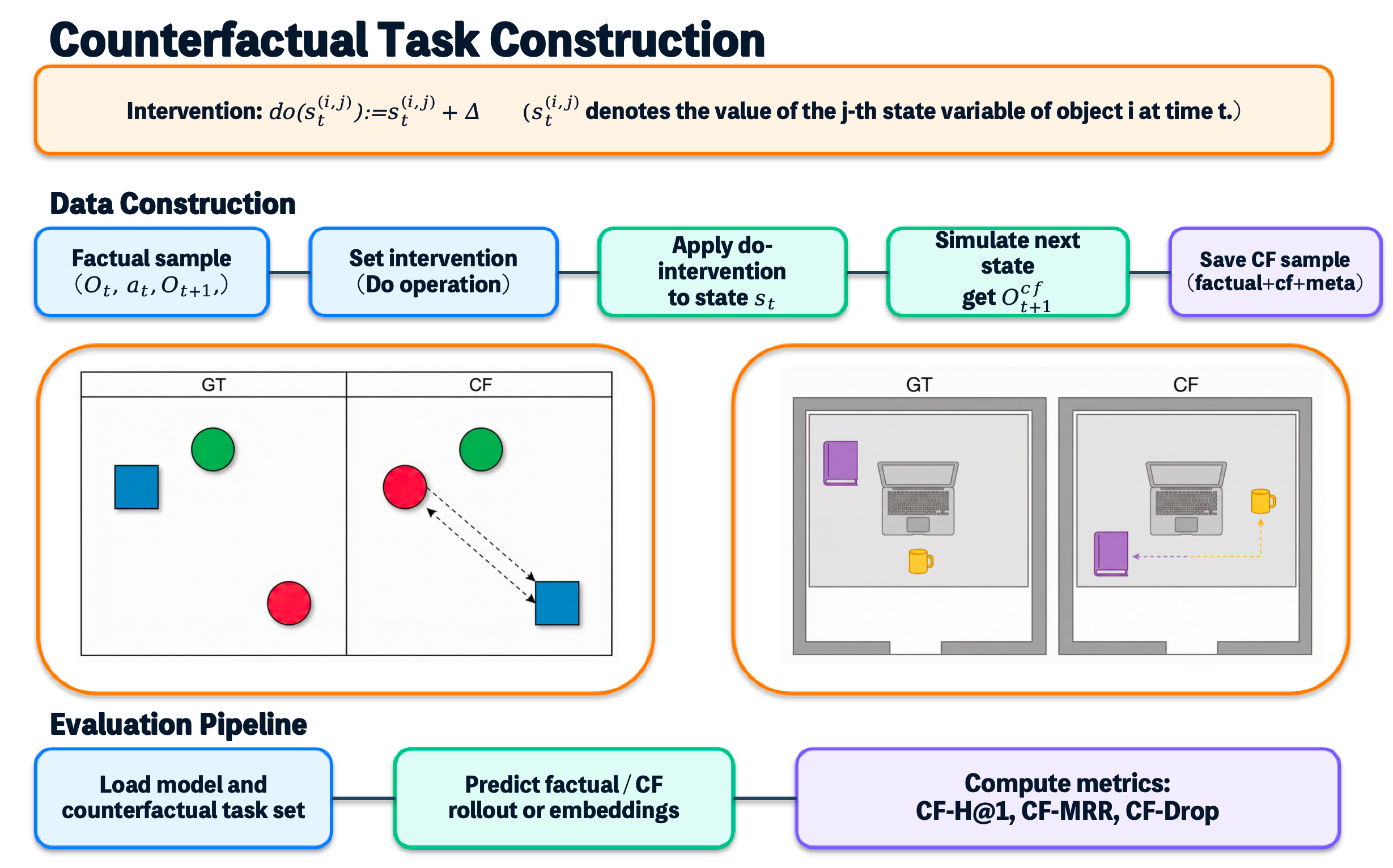
<p>We evaluate four domains—Physics 3-body, Chemistry, 2D Shapes, and 3D Cubes—using state-, object-, and mechanism-level interventions. Each factual transition is paired with a re-simulated counterfactual target.</p>

<figure class="figure">
  <a class="figure-image" aria-label="Counterfactual examples are created by applying a controlled do-intervention and re-simulating the next state. CF-H 1 and CF-MRR measure whether the model retrieves the correct alternative future.">
    <img src="/preview/pr-10/images/CausalVAE/counterfactual-task-construction.png" style="
        width: 100%;
        max-height: unset;
      " alt="Counterfactual examples are created by applying a controlled do-intervention and re-simulating the next state. CF-H 1 and CF-MRR measure whether the model retrieves the correct alternative future." loading="lazy" onerror="this.src = '/preview/pr-10/images/fallback.svg'; this.onerror = null;" />
  </a>
  
    <figcaption class="figure-caption">
      Counterfactual examples are created by applying a controlled do-intervention and re-simulating the next state. CF-H@1 and CF-MRR measure whether the model retrieves the correct alternative future.

    </figcaption>
  
</figure>

<p>The evaluation asks a direct question: among candidate futures, does the model retrieve the one produced by the intervention? Factual H@1 and MRR track ordinary prediction, while CF-H@1 and CF-MRR isolate counterfactual retrieval.</p>

<h2 id="the-largest-gains-appear-where-ordinary-dynamics-are-intervention-fragile">The largest gains appear where ordinary dynamics are intervention-fragile</h2>

<p>Across four benchmarks and eight paired backbones, the plug-in generally keeps factual retrieval competitive and improves CF-H@1 on <strong>21 of 32 backbone–benchmark pairs</strong>. Physics shows the clearest effect: GNN–NLL rises from <strong>11.0 to 41.0 CF-H@1</strong>, a gain of 30.0 points, while AE–NLL rises from <strong>10.5 to 41.0</strong>, a gain of 30.5 points.</p>

<table>
  <thead>
    <tr>
      <th>Physics 3-body backbone</th>
      <th style="text-align: right">Baseline CF-H@1</th>
      <th style="text-align: right">+ CausalVAE</th>
    </tr>
  </thead>
  <tbody>
    <tr>
      <td>AE · Contrastive</td>
      <td style="text-align: right">10.0</td>
      <td style="text-align: right">24.0</td>
    </tr>
    <tr>
      <td>AE · NLL</td>
      <td style="text-align: right">10.5</td>
      <td style="text-align: right">**41.0**</td>
    </tr>
    <tr>
      <td>VAE · Contrastive</td>
      <td style="text-align: right">8.5</td>
      <td style="text-align: right">8.5</td>
    </tr>
    <tr>
      <td>VAE · NLL</td>
      <td style="text-align: right">10.5</td>
      <td style="text-align: right">13.0</td>
    </tr>
    <tr>
      <td>Modular · Contrastive</td>
      <td style="text-align: right">22.5</td>
      <td style="text-align: right">25.0</td>
    </tr>
    <tr>
      <td>Modular · NLL</td>
      <td style="text-align: right">14.5</td>
      <td style="text-align: right">22.0</td>
    </tr>
    <tr>
      <td>GNN · Contrastive</td>
      <td style="text-align: right">11.5</td>
      <td style="text-align: right">15.0</td>
    </tr>
    <tr>
      <td>GNN · NLL</td>
      <td style="text-align: right">11.0</td>
      <td style="text-align: right">**41.0**</td>
    </tr>
  </tbody>
</table>

<p>In the matched Physics comparison, the plug-in adds approximately 1M parameters.</p>

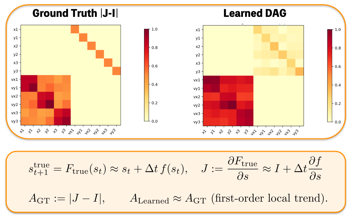
<p>The learned structure is also interpretable at the mechanism-trend level. On Physics, its strongest edges align with a first-order template derived from the locally linearized dynamics. This is evidence of meaningful physical interaction trends—not a claim that a local DAG exactly recovers the full nonlinear law.</p>

<figure class="figure">
  <a class="figure-image" aria-label="The learned adjacency recovers the main first-order interaction pattern of the Physics system. The comparison is local and approximate by design.">
    <img src="/preview/pr-10/images/CausalVAE/gt-vs-learned.png" style="
        width: min(100%, 860px);
        max-height: unset;
      " alt="The learned adjacency recovers the main first-order interaction pattern of the Physics system. The comparison is local and approximate by design." loading="lazy" onerror="this.src = '/preview/pr-10/images/fallback.svg'; this.onerror = null;" />
  </a>
  
    <figcaption class="figure-caption">
      The learned adjacency recovers the main first-order interaction pattern of the Physics system. The comparison is local and approximate by design.

    </figcaption>
  
</figure>

<h2 id="where-the-plug-in-breaks-the-host-latent-still-matters">Where the plug-in breaks: the host latent still matters</h2>

<p>The gains are not universal. Chemistry exposes a capacity bottleneck: some backbones compress <code class="language-plaintext highlighter-rouge">5^5 = 3,125</code> global color configurations into a five-dimensional code. Passing that code through another structured encode–decode path can erase class-discriminative directions. In this setting, causal regularization has too little representational room to help.</p>

<p>For AE–Contrastive on Chemistry, increasing the latent dimension changes the CF-H@1 gain monotonically:</p>

<table>
  <thead>
    <tr>
      <th>Latent dimension</th>
      <th style="text-align: right">5</th>
      <th style="text-align: right">16</th>
      <th style="text-align: right">32</th>
      <th style="text-align: right">128</th>
    </tr>
  </thead>
  <tbody>
    <tr>
      <td>CF-H@1 change</td>
      <td style="text-align: right">−16.7</td>
      <td style="text-align: right">−9.2</td>
      <td style="text-align: right">−1.5</td>
      <td style="text-align: right">+3.5</td>
    </tr>
  </tbody>
</table>

<p>The practical lesson is specific: use the plug-in when the backbone latent can still carry the relevant causal factors, and validate it per domain. Long-horizon drift and strongly nonlinear regimes remain open problems.</p>

<h2 id="the-takeaway">The takeaway</h2>

<div class="alert" style="--color: #0ea5e9">
  
  <i class="icon fa-solid fa-circle-info"></i>
  <div class="alert-content">
    <p><strong>Structure can be added without starting over.</strong> Keep the predictive backbone, organize its latent variables, and train the causal bridge carefully. Where ordinary dynamics confuse correlation with mechanism, explicit causal structure can make the alternative future much easier to find.</p>

  </div>
</div>

<p><a href="https://arxiv.org/pdf/2604.07712">Read the ECCV 2026 paper</a></p>]]></content><author><name>Ziyi Ding</name></author><category term="publication" /><category term="world-models" /><category term="causal-learning" /><category term="counterfactuals" /><summary type="html"><![CDATA[Predicting Is Not Yet Understanding]]></summary><media:thumbnail xmlns:media="http://search.yahoo.com/mrss/" url="/preview/pr-10/images/CausalVAE/method-overview.png" /><media:content medium="image" url="/preview/pr-10/images/CausalVAE/method-overview.png" xmlns:media="http://search.yahoo.com/mrss/" /></entry><entry><title type="html">CWI — Composite Humanoid Whole-Body Imitation System for Loco-Manipulation (RA-L 2026)</title><link href="/preview/pr-10/2026/08/04/CWI-blog.html" rel="alternate" type="text/html" title="CWI — Composite Humanoid Whole-Body Imitation System for Loco-Manipulation (RA-L 2026)" /><published>2026-08-04T00:00:00+00:00</published><updated>2026-10-10T14:58:01+00:00</updated><id>/preview/pr-10/2026/08/04/CWI-blog</id><content type="html" xml:base="/preview/pr-10/2026/08/04/CWI-blog.html"><![CDATA[<h3 id="one-policy-two-kinds-of-motion-data">One Policy, Two Kinds of Motion Data</h3>

<p><em>Accepted to IEEE Robotics and Automation Letters, June 2026.</em></p>

<p>Wenqi Ge*, Junde Guo*, Zhen Fu, Shunpeng Yang, Jiayu Chen, Hua Chen</p>

<p>LimX Dynamics · The University of Hong Kong · SUSTech · HKUST · Zhejiang University</p>

<p><sub>*Equal contribution</sub></p>

<p><a href="https://cwi-ral.github.io/CWI-RAL-Webpage/">Project page</a> · <a href="https://arxiv.org/abs/2606.27676">arXiv:2606.27676</a> · <a href="https://youtu.be/BLckpzHSI0w">Video (YouTube)</a> · <a href="https://www.bilibili.com/video/BV1dzKf6GEeH/">Video (Bilibili)</a></p>

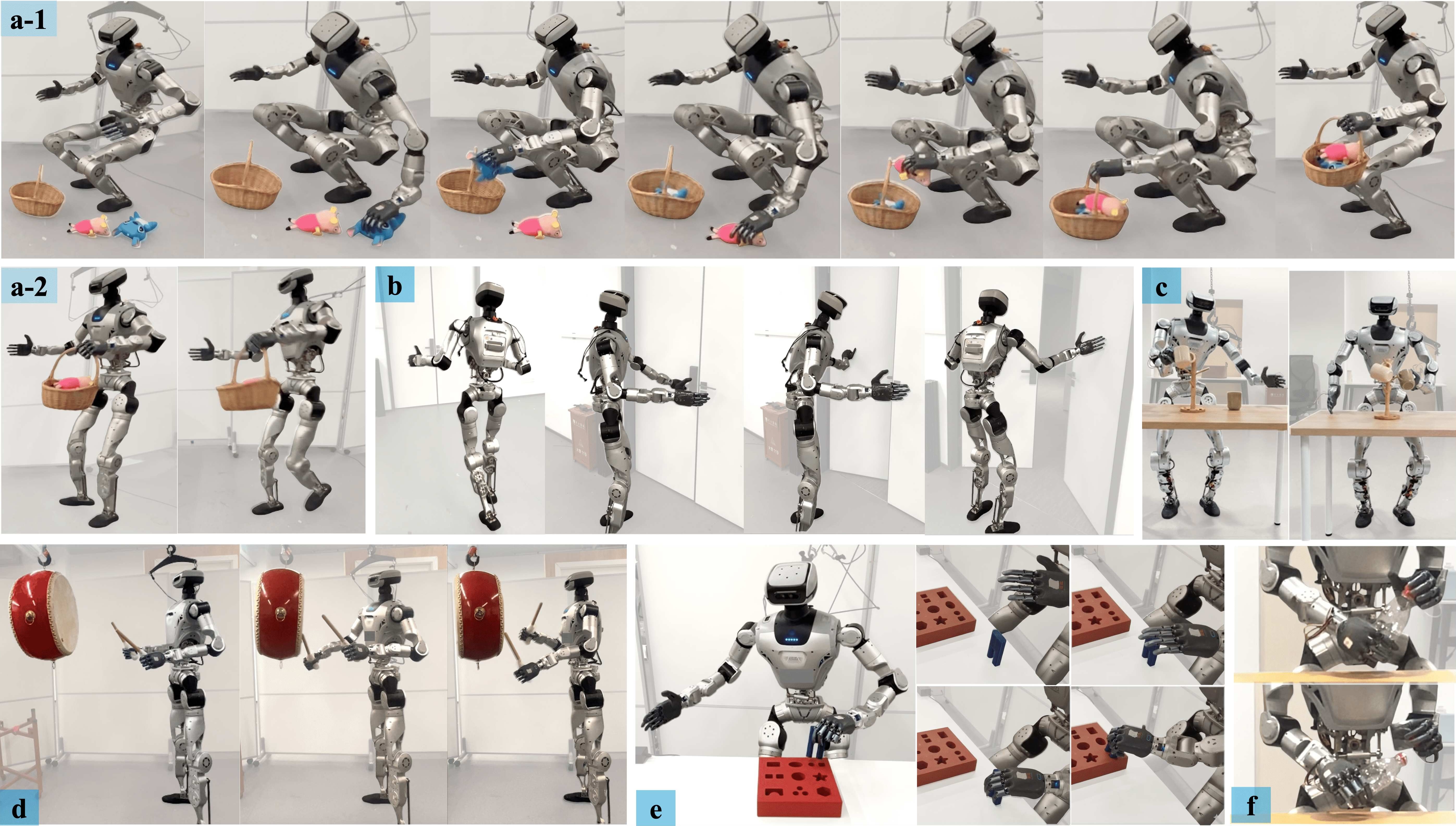
<p><img src="/images/CWI/fig1-tasks.jpg" alt="Seven real-world loco-manipulation tasks performed by a LimX Oli humanoid under CWI" /></p>

<p><em>CWI on a full-size LimX Oli: squatting to pick up toys and drop them in a basket (a-1), standing up and walking off carrying it (a-2), opening a door (b), hanging cups on a rack (c), striking a suspended drum (d), assembling a small part (e), twisting a bottle cap (f).</em></p>

<p>A humanoid that picks a toy off the floor and carries it across the room is solving two problems at once. The legs have to hold a commanded velocity and height while the arms swing the base around. The arms have to reach wherever the operator points, with motion that stays inside what a human body would actually produce. Push hard on one objective and the other tends to give.</p>

<p>Human motion capture is the obvious source of priors for both halves. That is also where the trouble starts.</p>

<h2 id="where-full-body-mocap-breaks-down">Where full-body MoCap breaks down</h2>

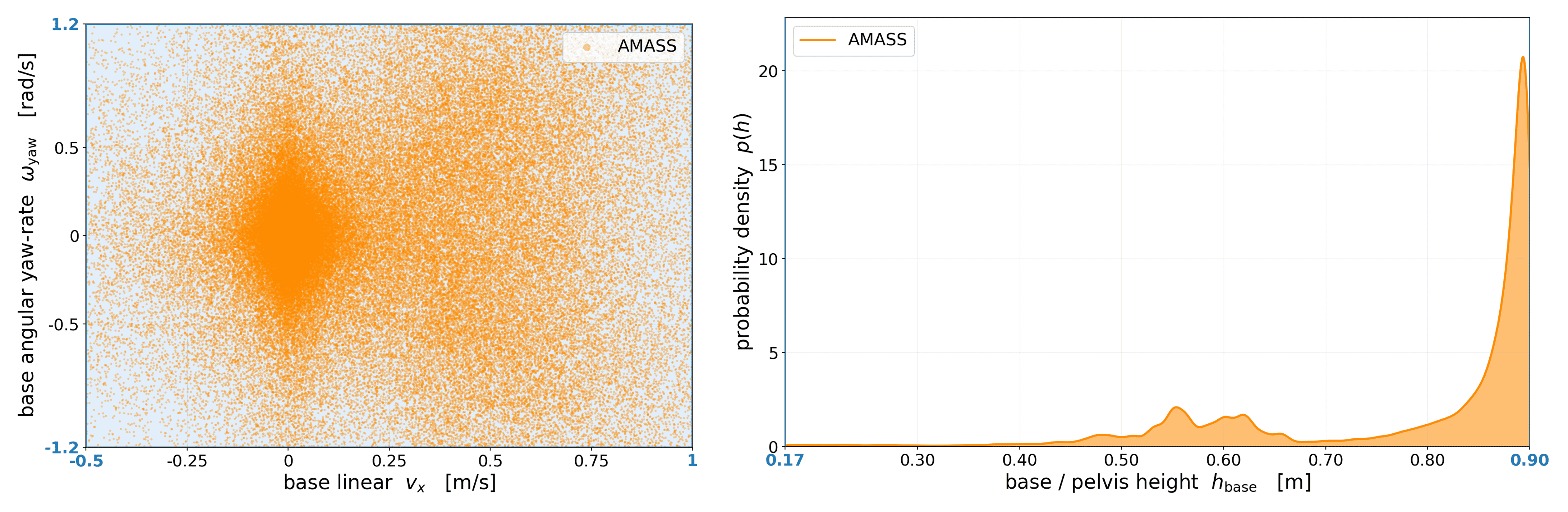
<p>AMASS and similar corpora are not evenly useful across the body. Upper-body trajectories are rich: people reach, gesture, and handle objects in every direction, which is close to what a manipulation policy needs. Lower-body trajectories are another matter.</p>

<p><img src="/images/CWI/fig3-amass-distribution.png" alt="Left: pelvis-height density in AMASS peaks near 0.85 to 0.90 m. Right: base linear and angular velocity scatter clusters near the origin" /></p>

<p><em>AMASS lower-body statistics against our training command range (blue). Pelvis height piles up near standing, 0.85 to 0.90 m, while we command down to 0.17 m. Base velocities cluster at the origin, while we command up to 1.0 m/s forward and 1.2 rad/s in yaw.</em></p>

<p>Two things go wrong. The clips do not cover the corners of the command box we need for deployment, so a policy trained to track them never learns to hold 0.3 m/s at a 0.4 m squat. And many of the clips that do move are too aggressive for a robot that is carrying something, so they have to be filtered out.</p>

<p>Both standard responses to this cost something. Filtering the corpus for lower-body stability throws away the upper-body motion in those same clips, which was perfectly good. Skipping MoCap for the legs and shaping rewards or sampling joint commands instead leaves the upper body without human statistics, and the arm motion drifts away from anything a person would produce.</p>

<h2 id="decouple-the-data-keep-the-policy-whole">Decouple the data, keep the policy whole</h2>

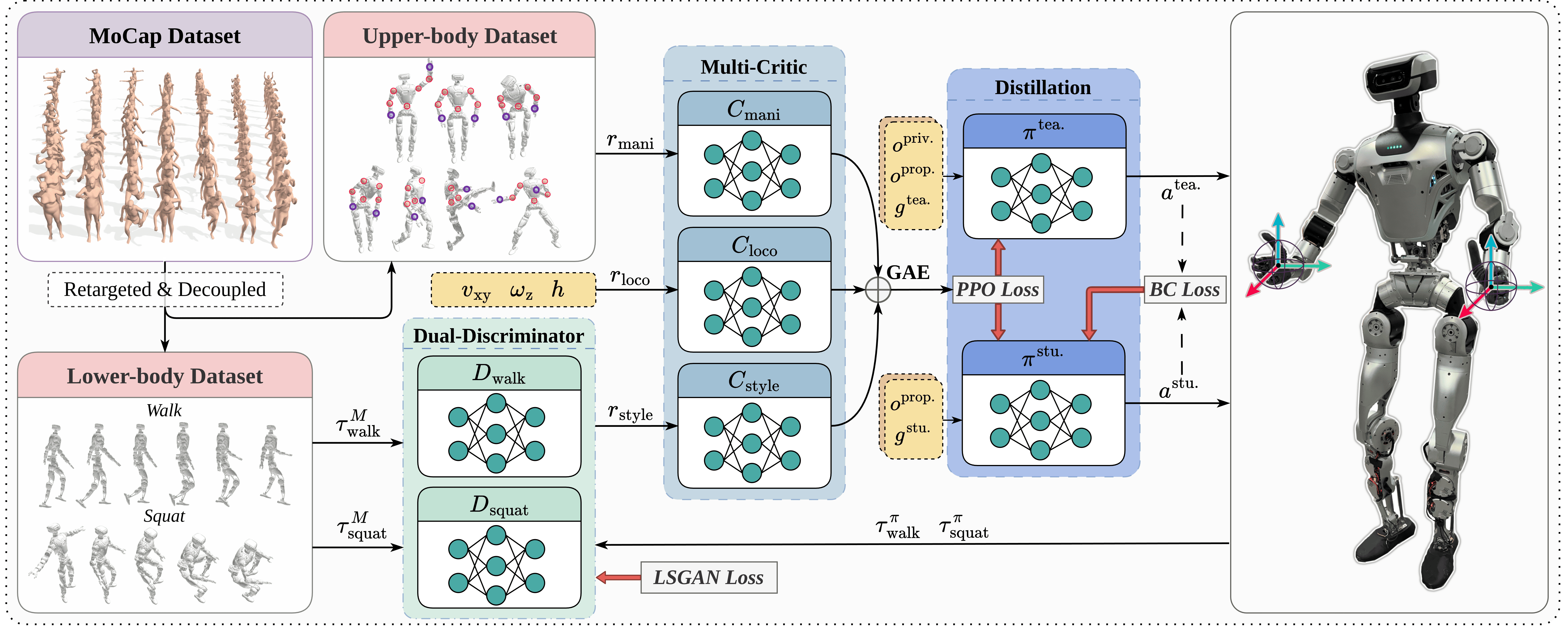
<p>Several existing loco-manipulation controllers decouple the <em>architecture</em>: one policy for the legs and another for the arms, or RL for the legs and PD control on top for the arms. CWI keeps a single whole-body policy over all 31 DoF and decouples only what each half learns from.</p>

<p>The upper body trains on the full AMASS corpus with no filtering. The lower body trains on roughly ten curated expert-quality clips per class, one class for omnidirectional walking and one for squatting.</p>

<p><img src="/images/CWI/fig2-framework.png" alt="CWI framework overview showing decoupled data sources, dual AMP discriminators, multi-critic PPO, and teacher-student distillation" /></p>

<p><em>The CWI framework. Large-scale upper-body data drives manipulation, compact curated clips drive locomotion style through two discriminators, a multi-critic PPO stage trains the unified policy, and distillation produces a student driven by velocity/height commands plus bimanual hand poses.</em></p>

<p>The reason the upper-body corpus needs no filtering is a change of frame. We express every upper-body reference relative to the robot’s base. Once root motion is subtracted, a clip of someone spinning or jumping still contains a clean, human-feasible arm trajectory. The instability lives in the root, and the root is exactly what we drop.</p>

<p>Two details in how the body is partitioned turn out to matter later. The waist (yaw, roll, pitch) goes into the upper-body group, so torso bending is supervised by the same AMASS clip as the arms rather than being treated as part of the locomotion problem. The neck and head come out of the reference entirely, since AMASS contains very few head motions; instead the head gets a 2-DoF command sampled within its mechanical range each episode and a separate quadratic tracking term, which lets a VR headset drive it directly at deployment.</p>

<p>The upper-body reference combines joint targets <code class="language-plaintext highlighter-rouge">q_u^ref ∈ R^17</code> with position, orientation, and keypoint-based pose for the shoulder, elbow, wrist, and hand links. The lower-body reference for the discriminators carries base velocity and height, the 12 leg joint positions and velocities, and hip/knee/ankle link states.</p>

<h2 id="two-discriminators-one-per-gait-class">Two discriminators, one per gait class</h2>

<p>The lower body gets its supervision through Adversarial Motion Priors rather than frame-by-frame tracking. Each discriminator scores a four-frame window of lower-body state transitions, with upper-body signals excluded so the prior stays purely about the legs, and trains with a least-squares GAN objective plus a gradient penalty.</p>

<p>Which discriminator is active depends on the command: <code class="language-plaintext highlighter-rouge">D_walk</code> when the velocity command is nonzero, <code class="language-plaintext highlighter-rouge">D_squat</code> when it is zero and the policy is tracking height. Both feed a continuous style reward that pays off states the discriminator classifies as expert-like.</p>

<p>The important consequence is that the curated clips act as a style prior, not a tracking target. Locomotion commands are sampled uniformly across the entire deployment range during training, far outside anything the ten clips demonstrate. The discriminator answers “does this look like expert walking”, not “does this match frame 47 of clip 3”, so command coverage and motion quality stop competing for the same data.</p>

<p>Walking and squatting are distinct enough that pooling them into one discriminator averages the two modes and blurs both, which the ablations below confirm.</p>

<h2 id="three-reward-groups-three-critics">Three reward groups, three critics</h2>

<p>The full reward splits into locomotion tracking, upper-body tracking, and style:</p>

<table>
  <thead>
    <tr>
      <th>Group</th>
      <th>Term</th>
      <th>Definition</th>
      <th>Weight</th>
    </tr>
  </thead>
  <tbody>
    <tr>
      <td><code class="language-plaintext highlighter-rouge">r_loco</code></td>
      <td>Linear velocity</td>
      <td><code class="language-plaintext highlighter-rouge">exp(−(v_xy − v_xy^cmd)²)</code></td>
      <td>3.0</td>
    </tr>
    <tr>
      <td> </td>
      <td>Angular velocity</td>
      <td><code class="language-plaintext highlighter-rouge">exp(−(ω_z − ω_z^cmd)²)</code></td>
      <td>2.5</td>
    </tr>
    <tr>
      <td> </td>
      <td>Height tracking</td>
      <td><code class="language-plaintext highlighter-rouge">exp(−(h − h^cmd)²)</code></td>
      <td>2.5</td>
    </tr>
    <tr>
      <td><code class="language-plaintext highlighter-rouge">r_upper</code></td>
      <td>DoF position</td>
      <td><code class="language-plaintext highlighter-rouge">exp(−‖q_upper − q_ref^upper‖²/σ_q²)</code></td>
      <td>2.0</td>
    </tr>
    <tr>
      <td> </td>
      <td>Tri-keypoint position</td>
      <td><code class="language-plaintext highlighter-rouge">exp(−‖p̃_u − p̃_ref^upper‖²/σ_p²)</code></td>
      <td>3.0</td>
    </tr>
    <tr>
      <td><code class="language-plaintext highlighter-rouge">r_style</code></td>
      <td>AMP</td>
      <td><code class="language-plaintext highlighter-rouge">max(0, 1 − 0.25(D_φ^k(τ) − 1)²)</code></td>
      <td>2.0</td>
    </tr>
  </tbody>
</table>

<p>Standard regularizers (projected-gravity alignment, action smoothness, torque penalties) are assigned to whichever group they primarily affect.</p>

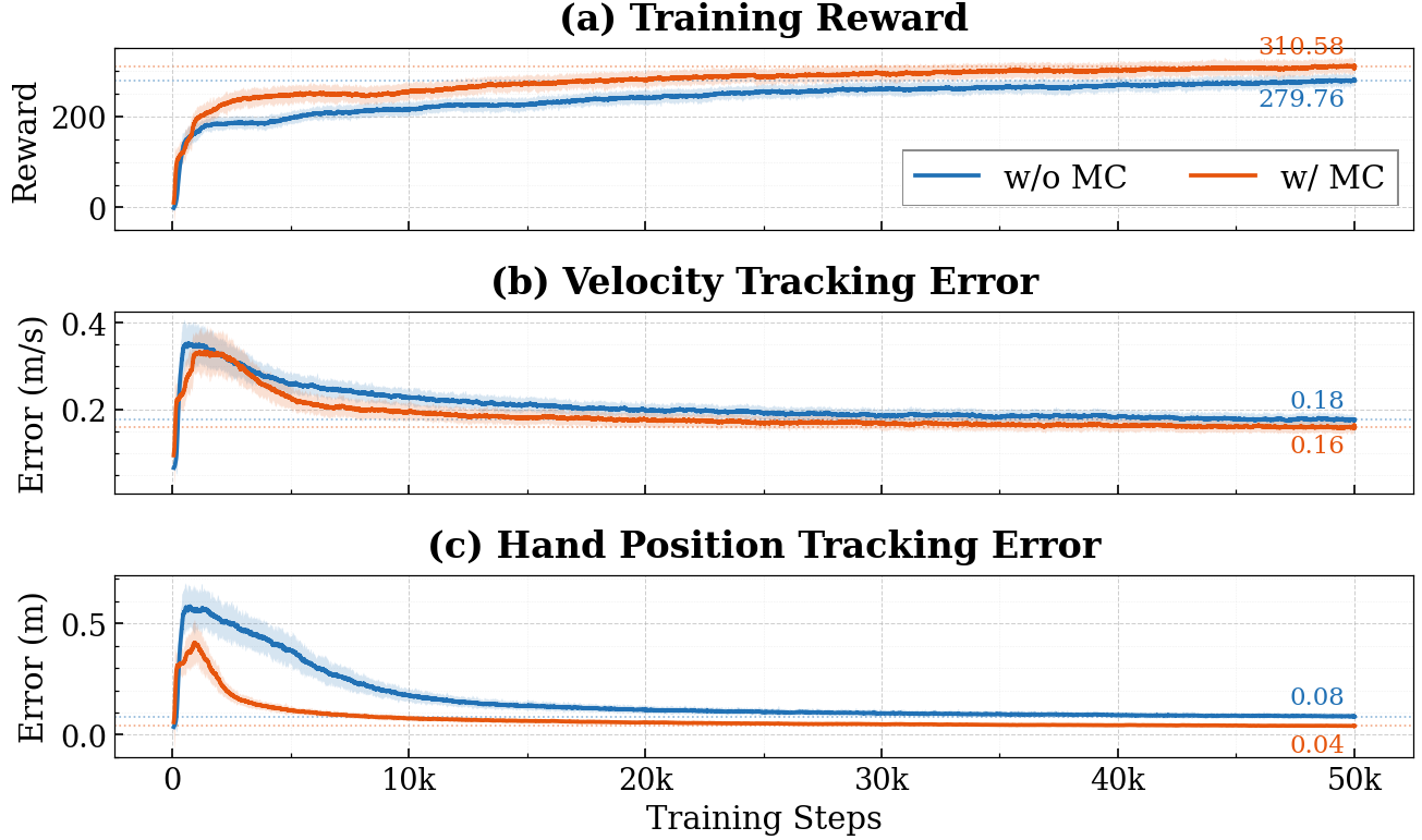
<p>A single critic has to explain all three signals with one value function, and the adversarial style reward is high-variance enough to drag that estimate around. We give each group its own value head, compute group-wise GAE advantages, normalize each within the minibatch, and combine them with weights before the standard PPO clipped surrogate.</p>

<p><img src="/images/CWI/fig5-multicritic-curves.png" alt="Training curves for single-critic and multi-critic variants, showing reward, velocity tracking error, and hand position tracking error" /></p>

<p><em>The multi-critic variant reaches a higher final reward and converges faster on both velocity and hand-position error.</em></p>

<h2 id="distilling-down-to-two-hand-poses">Distilling down to two hand poses</h2>

<p>Single-stage RL for whole-body tracking tends to come out jerky, so we train a teacher with privileged state and the full upper-body reference, then distill.</p>

<p>The student sees only a history of proprioceptive observations plus a reduced command: velocity and height for the legs, and an 18-dimensional bimanual hand pose (a 9D keypoint feature per hand) for the arms. Distillation combines PPO on the teacher’s reward with an action-matching BC term, querying the teacher on-policy over the student’s own state distribution and annealing the imitation weight.</p>

<p>Reducing the command to hand poses is a deployment decision. A VR operator supplies end-effector targets, not joint angles, and reconstructing joint targets through online IK risks discontinuities near singularities. Distilling directly on hand poses sidesteps that and keeps the student pinned to the AMASS manifold. The cost is a small open-loop accuracy gap against the joint-command interface.</p>

<h2 id="how-it-compares">How it compares</h2>

<p>We evaluate on a 31-DoF LimX Oli (1.65 m, 50 kg), trained in IsaacLab with commands sampled over <code class="language-plaintext highlighter-rouge">v_x ∈ [−0.5, 1.0]</code> m/s, <code class="language-plaintext highlighter-rouge">ω_yaw ∈ [−1.2, 1.2]</code> rad/s, <code class="language-plaintext highlighter-rouge">h ∈ [0.17, 0.9]</code> m, and the usual domain randomization over mass, friction, sensor noise, and latency. The AMASS upper-body corpus is split 85/15, and evaluation uses sequences the policy never saw.</p>

<p>Because the original works target different robots, we re-implemented every baseline on Oli (marked with *) and unified observation composition, reward terms and weights, and PD gains across all methods, so the comparison isolates framework design and data usage.</p>

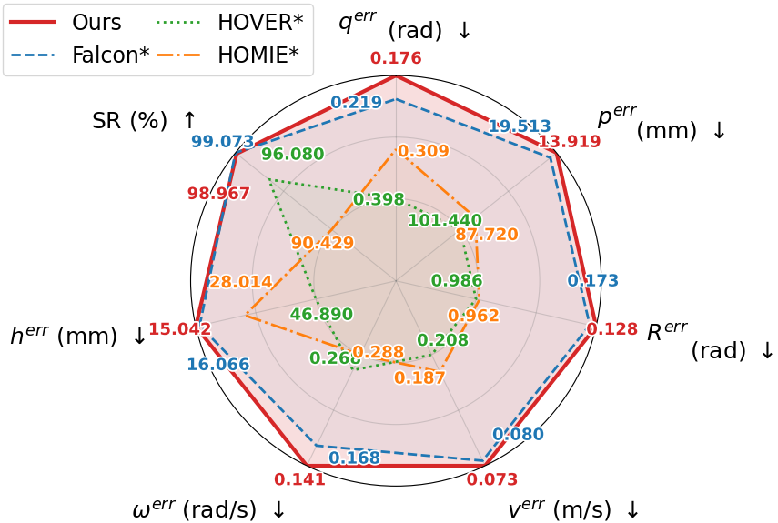
<p><img src="/images/CWI/fig4-comparison-radar.png" alt="Radar chart comparing CWI against FALCON*, HOMIE*, and HOVER* across seven metrics" /></p>

<table>
  <thead>
    <tr>
      <th>Metric</th>
      <th>CWI (ours)</th>
      <th>FALCON*</th>
      <th>HOMIE*</th>
      <th>HOVER*</th>
    </tr>
  </thead>
  <tbody>
    <tr>
      <td>Success rate (%)</td>
      <td>98.967</td>
      <td>**99.073**</td>
      <td>90.429</td>
      <td>96.080</td>
    </tr>
    <tr>
      <td>Upper-body joint error (rad)</td>
      <td>**0.176**</td>
      <td>0.219</td>
      <td>0.309</td>
      <td>0.398</td>
    </tr>
    <tr>
      <td>Keybody position error (mm)</td>
      <td>**13.919**</td>
      <td>19.513</td>
      <td>87.720</td>
      <td>101.440</td>
    </tr>
    <tr>
      <td>Keybody orientation error (rad)</td>
      <td>**0.128**</td>
      <td>0.173</td>
      <td>0.962</td>
      <td>0.986</td>
    </tr>
    <tr>
      <td>Linear velocity error (m/s)</td>
      <td>**0.073**</td>
      <td>0.080</td>
      <td>0.187</td>
      <td>0.208</td>
    </tr>
    <tr>
      <td>Yaw rate error (rad/s)</td>
      <td>**0.141**</td>
      <td>0.168</td>
      <td>0.288</td>
      <td>0.260</td>
    </tr>
    <tr>
      <td>Height error (mm)</td>
      <td>**15.042**</td>
      <td>16.066</td>
      <td>28.014</td>
      <td>46.890</td>
    </tr>
  </tbody>
</table>

<p><em>Lower is better on every row except success rate. Position and orientation errors aggregate over all upper-body keypoints.</em></p>

<p>FALCON* carries higher arm tracking error, consistent with its separate upper and lower policies. HOVER* loses robustness once upper-body motions are paired with base commands outside its training distribution. HOMIE* shows larger joint-level deviation, which fits a PD-controlled upper body asked to follow non-smooth references.</p>

<p>The one metric where CWI does not come first is success rate, where FALCON* leads by about a tenth of a percentage point. Our policy holds strict upper-body tracking even at the boundary of the command box, and that occasionally costs a little stability.</p>

<h2 id="which-pieces-are-doing-the-work">Which pieces are doing the work</h2>

<p>The ablations use the deployment-interface student, so the manipulation columns report end-effector error over the two hands rather than the full-keypoint aggregate above. We add a relaxed DTW distance <code class="language-plaintext highlighter-rouge">d_dtw</code> against reference clips as a naturalness measure, and the 95th-percentile joint acceleration <code class="language-plaintext highlighter-rouge">q̈_p95</code> as a smoothness proxy.</p>

<table>
  <thead>
    <tr>
      <th>Variant</th>
      <th>v error (m/s)</th>
      <th>ω error (rad/s)</th>
      <th>h error (mm)</th>
      <th>EE pos (mm)</th>
      <th>EE rot (rad)</th>
      <th>d_dtw (rad)</th>
      <th>q̈_p95 (rad/s²)</th>
    </tr>
  </thead>
  <tbody>
    <tr>
      <td>CWI (full)</td>
      <td>0.100</td>
      <td>**0.1825**</td>
      <td>**19.65**</td>
      <td>**42.91**</td>
      <td>0.1708</td>
      <td>**0.452**</td>
      <td>**28.8**</td>
    </tr>
    <tr>
      <td>w/o multi-critic</td>
      <td>**0.099**</td>
      <td>0.199</td>
      <td>20.64</td>
      <td>55.49</td>
      <td>0.2308</td>
      <td>0.520</td>
      <td>30.4</td>
    </tr>
    <tr>
      <td>w/o distillation †</td>
      <td>0.099</td>
      <td>0.147</td>
      <td>19.43</td>
      <td>173.2</td>
      <td>0.6723</td>
      <td>0.444</td>
      <td>28.1</td>
    </tr>
    <tr>
      <td>single AMP</td>
      <td>0.110</td>
      <td>0.192</td>
      <td>21.07</td>
      <td>42.93</td>
      <td>0.1702</td>
      <td>0.615</td>
      <td>35.1</td>
    </tr>
    <tr>
      <td>w/o AMP</td>
      <td>0.125</td>
      <td>0.242</td>
      <td>22.52</td>
      <td>42.92</td>
      <td>**0.1696**</td>
      <td>1.413</td>
      <td>39.3</td>
    </tr>
    <tr>
      <td>w/o AMASS upper</td>
      <td>0.131</td>
      <td>0.249</td>
      <td>24.20</td>
      <td>62.32</td>
      <td>0.275</td>
      <td>0.508</td>
      <td>48.2</td>
    </tr>
  </tbody>
</table>

<p><sub>† The single-stage variant fails upper-body tracking outright, so its locomotion numbers are reported for transparency but not ranked.</sub></p>

<p>Removing distillation is the sharpest failure. A single-stage policy cannot learn manipulation from the sparse hand-pose command alone, and end-effector error goes from 42.91 mm to 173.2 mm. The teacher has to learn whole-body control with dense references first; the student inherits it.</p>

<p>Dropping AMP barely touches command tracking but collapses gait quality: <code class="language-plaintext highlighter-rouge">d_dtw</code> jumps from 0.452 to 1.413 rad, with frequent stance violations and foot slips. Pooling the two discriminators into one is the same failure in milder form, with <code class="language-plaintext highlighter-rouge">d_dtw</code> at 0.615 and joint acceleration up from 28.8 to 35.1 rad/s². End-effector accuracy stays near 42.9 mm in both cases, so the dual-discriminator design buys lower-body style without charging manipulation for it.</p>

<p>The result we find most telling is the AMASS upper-body ablation. Swapping human references for randomly sampled joint targets degrades manipulation as expected (42.91 to 62.32 mm, joint acceleration 28.8 to 48.2 rad/s²), but it also degrades <em>every locomotion metric</em>: velocity error 0.100 to 0.131 m/s, yaw rate 0.183 to 0.249 rad/s, height 19.65 to 24.20 mm. The architecture supplies the structural decoupling. Only the data supplies upper-body motion whose statistics the legs can absorb, and a jerky upper body is a disturbance the legs then have to reject.</p>

<h2 id="on-the-robot">On the robot</h2>

<p>Deployment runs off a Meta Quest headset and its hand controllers, with no MoCap suit and no exoskeleton cockpit. The operator’s hand poses and a velocity/height command are the entire interface.</p>

<p>The tasks in the opening figure cover precision work (twisting a bottle cap, assembling a small part), whole-body coordination (opening a door, striking a suspended drum), and long-horizon sequences (picking up toys, placing them, then carrying the basket away). The policy holds stable locomotion throughout.</p>

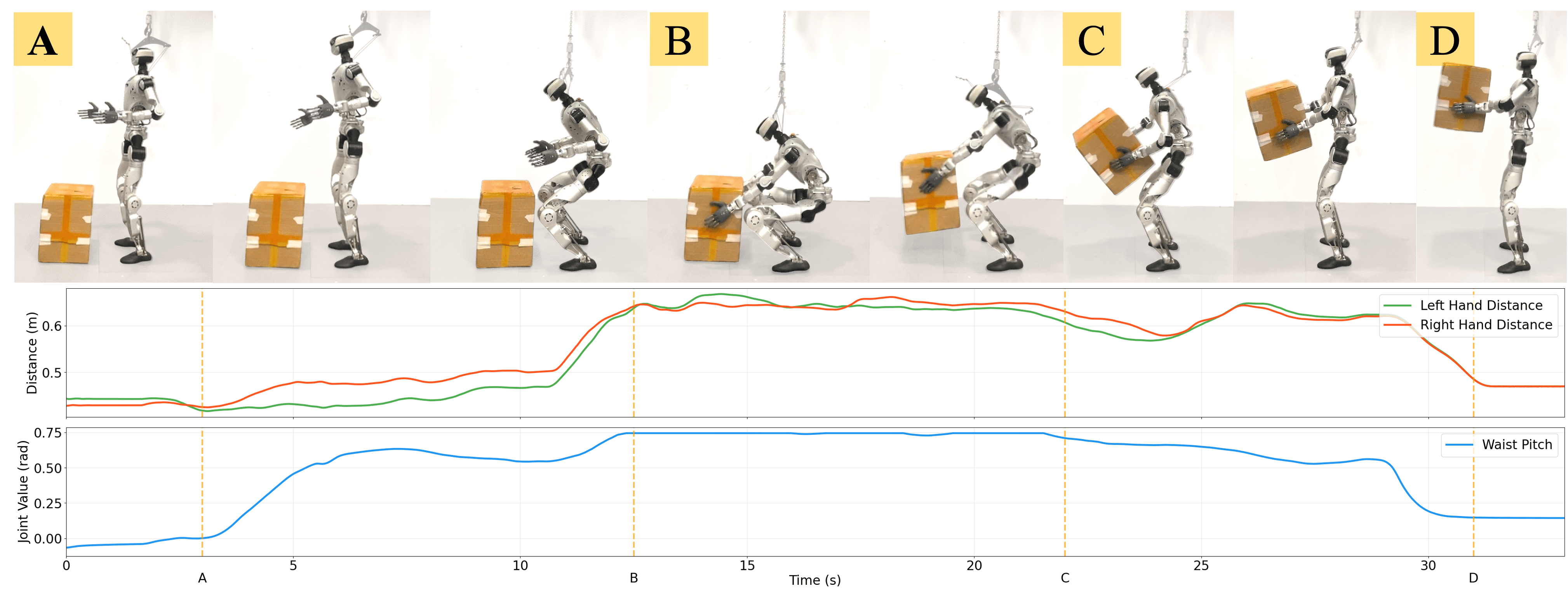
<p><img src="/images/CWI/fig6-box-lifting-coordination.png" alt="Box-lifting sequence with hand distance and waist pitch plotted over four phases" /></p>

<p><em>Four phases of a teleoperated box lift: approaching and squatting (A), grasping and starting the lift (B), raising with both hands (C), standing up with the box overhead (D). Below, left and right hand distance from the base against waist pitch over time.</em></p>

<p>Watch the waist pitch. It rises as the hands extend forward and down, then straightens as the robot comes upright with the box. The operator never sent a torso command; there is no torso command in the interface. The coupling between hand reach and torso posture is in the AMASS clips because that is how people reach, and putting the waist in the upper-body group meant one clip supervised both. The composite objective keeps that coupling intact while the legs stay stable underneath it.</p>

<h2 id="limits-and-what-comes-next">Limits and what comes next</h2>

<p>Behavior coverage is bounded by the motion libraries and, more tightly, by the command interface. Bimanual hand poses plus velocity and height cannot express pressing a pedal with a foot or bracing against a surface with an elbow.</p>

<p>That same compactness is useful going forward. A portable teleoperation rig that works in ordinary rooms is a data collection instrument, and a small, task-oriented command space is structured supervision for higher-level autonomous policies, vision-language-action models included. Collecting multimodal demonstrations in everyday scenes is where we are taking this next.</p>

<hr />

<h2 id="citation">Citation</h2>

<div class="language-bibtex highlighter-rouge"><div class="highlight"><pre class="highlight"><code><span class="nc">@article</span><span class="p">{</span><span class="nl">ge2026cwi</span><span class="p">,</span>
  <span class="na">author</span>  <span class="p">=</span> <span class="s">{Ge, Wenqi and Guo, Junde and Fu, Zhen and Yang, Shunpeng
             and Chen, Jiayu and Chen, Hua}</span><span class="p">,</span>
  <span class="na">title</span>   <span class="p">=</span> <span class="s">{{CWI}: Composite Humanoid Whole-Body Imitation System
             for Loco-Manipulation}</span><span class="p">,</span>
  <span class="na">journal</span> <span class="p">=</span> <span class="s">{IEEE Robotics and Automation Letters}</span><span class="p">,</span>
  <span class="na">year</span>    <span class="p">=</span> <span class="s">{2026}</span><span class="p">,</span>
  <span class="na">doi</span>     <span class="p">=</span> <span class="s">{10.1109/LRA.2026.3710366}</span>
<span class="p">}</span>
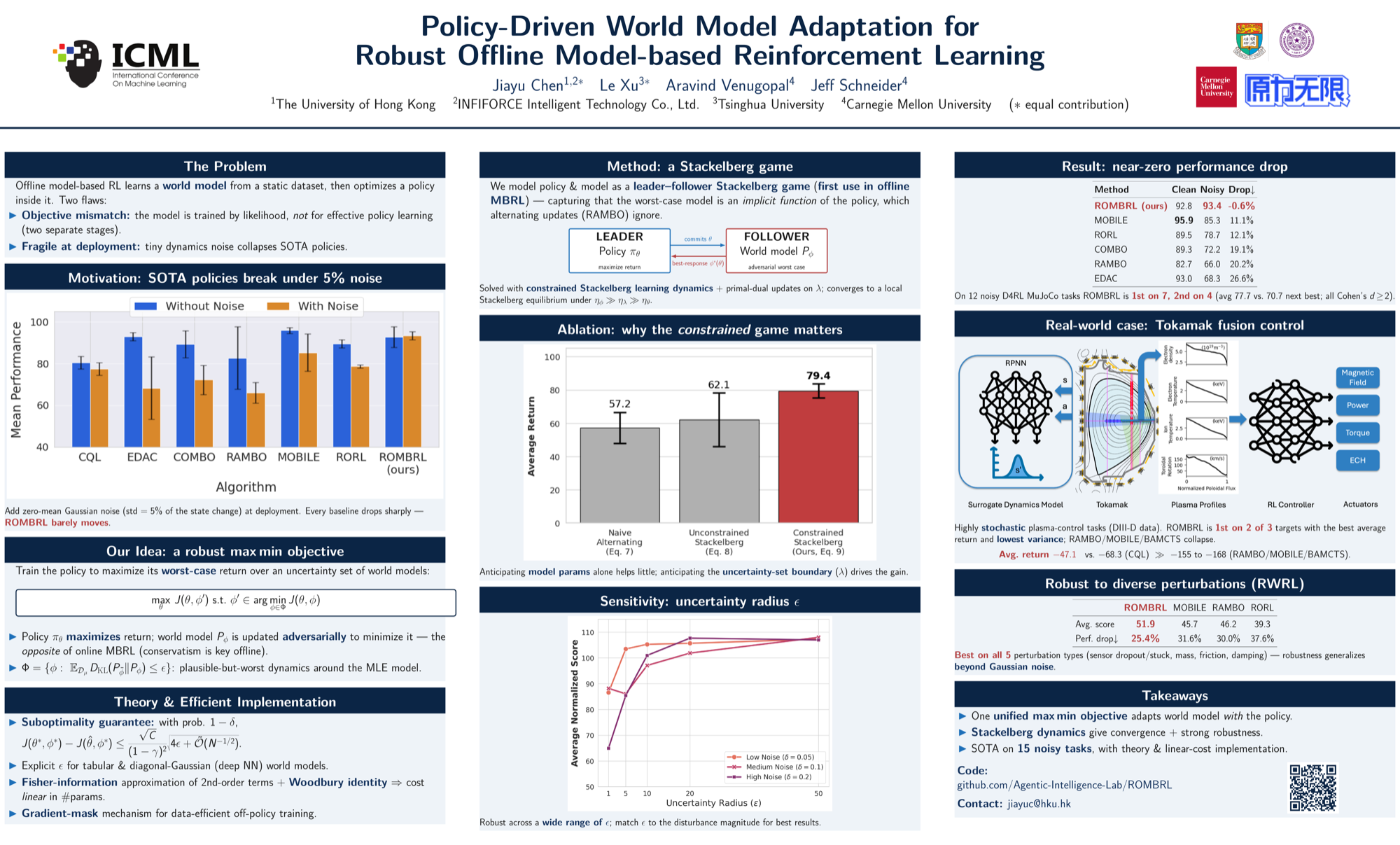
</code></pre></div></div>]]></content><author><name>Wenqi Ge</name></author><category term="publication" /><category term="robotics" /><category term="humanoid" /><category term="loco-manipulation" /><summary type="html"><![CDATA[One Policy, Two Kinds of Motion Data]]></summary><media:thumbnail xmlns:media="http://search.yahoo.com/mrss/" url="/preview/pr-10/images/CWI/fig1-tasks.jpg" /><media:content medium="image" url="/preview/pr-10/images/CWI/fig1-tasks.jpg" xmlns:media="http://search.yahoo.com/mrss/" /></entry><entry><title type="html">ROMBRL — Policy-Driven World Model Adaptation for Robust Offline Model-based RL (ICML 2026)</title><link href="/preview/pr-10/2026/08/04/rombrl-post.html" rel="alternate" type="text/html" title="ROMBRL — Policy-Driven World Model Adaptation for Robust Offline Model-based RL (ICML 2026)" /><published>2026-08-04T00:00:00+00:00</published><updated>2026-10-10T14:58:01+00:00</updated><id>/preview/pr-10/2026/08/04/rombrl-post</id><content type="html" xml:base="/preview/pr-10/2026/08/04/rombrl-post.html"><![CDATA[<p>Our paper, <strong>“Policy-Driven World Model Adaptation for Robust Offline Model-based Reinforcement Learning”</strong>, was presented as a <strong>poster at ICML 2026</strong> in Seoul, South Korea. This is joint work between the Agentic Intelligence Lab at the University of Hong Kong, Tsinghua University, and the Robotics Institute at Carnegie Mellon University.</p>

<ul>
  <li><strong>Paper (arXiv):</strong> <a href="https://arxiv.org/abs/2505.13709">arxiv.org/abs/2505.13709</a></li>
  <li><strong>OpenReview:</strong> <a href="https://openreview.net/forum?id=eB5i7caric">openreview.net/forum?id=eB5i7caric</a></li>
  <li><strong>Project page:</strong> <a href="https://agentic-intelligence-lab.github.io/ROMBRL/">agentic-intelligence-lab.github.io/ROMBRL</a></li>
  <li><strong>Code:</strong> <a href="https://github.com/Agentic-Intelligence-Lab/ROMBRL">github.com/Agentic-Intelligence-Lab/ROMBRL</a></li>
</ul>

<p><a href="/files/rombrl-poster.pdf" target="_blank">
  <img src="/images/rombrl-poster.png" alt="ROMBRL ICML 2026 poster" style="width:100%; max-width:100%; height:auto; border:1px solid #ddd;" />
</a></p>
<p style="text-align:center; font-size:0.9em; margin-top:-0.5em;"><em>Our ICML 2026 poster — click for the full-resolution PDF.</em></p>

<h2 id="tldr">TL;DR</h2>

<p>Offline model-based RL (MBRL) usually learns a world model and a policy in two separate stages — first fit the model to maximize data likelihood, then optimize the policy against the fixed model. This mismatch leaves policies brittle: even small amounts of deployment-time noise can wreck performance. We propose <strong>ROMBRL</strong>, which jointly adapts the world model <em>with</em> the policy under a single <strong>constrained maximin objective</strong>, solved via <strong>Stackelberg learning dynamics</strong> with the policy as the leader and the world model as an adversarial follower. ROMBRL comes with a formal suboptimality bound and achieves state-of-the-art robustness on D4RL MuJoCo and stochastic Tokamak Control benchmarks — with almost no cost to clean-environment performance.</p>

<h2 id="why-do-offline-rl-policies-fall-apart-under-a-little-noise">Why Do Offline RL Policies Fall Apart Under a Little Noise?</h2>

<p>Offline MBRL is appealing because it lets us train a policy from a static dataset by rolling it out inside a <em>learned</em> simulator, rather than the real environment — no risky exploration, no expensive interaction. But nearly all existing methods follow the same two-stage recipe: first fit a world model $P_\phi$ to maximize the likelihood of observed transitions, then freeze it (or only mildly adapt it) and optimize the policy $\pi_\theta$ against it.</p>

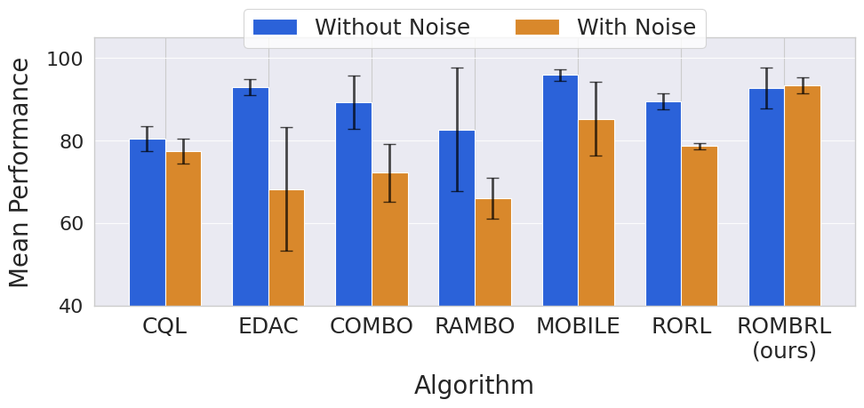
<p>That split has a quiet cost. The model is trained to <em>explain the data</em>, not to <em>support good policy learning</em> — an objective mismatch that’s easy to miss when you only evaluate in a clean, deterministic simulator. So we asked a more adversarial question: what happens to these policies once the environment doesn’t behave exactly like the simulator? We took a stable of strong offline RL baselines — CQL, EDAC, COMBO, MOBILE, and even RAMBO, which is specifically designed with an adversarial world model — and added just 5% Gaussian noise to state transitions at deployment time.</p>

<p><img src="/images/rombrl-fig1-motivation.png" alt="Average performance of offline RL algorithms before and after deployment noise" style="width:100%; max-width:600px; display:block; margin:1.5em auto;" /></p>
<p style="text-align:center; font-size:0.9em; margin-top:-1em;"><em>Average scores on nine D4RL MuJoCo tasks, before and after injecting 5% measurement noise at deployment. Every method — including the model-based robust baseline RAMBO — loses a substantial fraction of its performance.</em></p>

<p>Robustness, it turns out, is not something these methods get for free from good average returns.</p>

<h2 id="the-trick-turn-model-adaptation-into-an-adversarys-move">The Trick: Turn Model Adaptation Into an Adversary’s Move</h2>

<p>If the world model is going to be wrong somewhere, we’d rather it be wrong in a way our policy has already prepared for. That’s the intuition behind <strong>ROMBRL</strong>: instead of treating the world model as a fixed, passive stand-in for the environment, we make it move <em>against</em> the policy during training, so that whatever the policy learns has already survived a worst-case opponent.</p>

<p>Formally, we cast offline MBRL as a constrained maximin problem:</p>

<p>$$\max_\theta J(\theta, \phi’) \quad \text{s.t.} \quad \phi’ \in \arg\min_{\phi \in \Phi} J(\theta, \phi)$$</p>

<p>where $\Phi$ is an uncertainty set of world models $\phi \in \mathcal{M}$ anchored to the maximum-likelihood estimate $\hat\phi$ — a KL trust region around what the offline data actually supports:</p>

<p>$$\mathbb{E}_{(s,a)\sim\mathcal{D}}\left[ \mathrm{KL}\left(P_{\hat\phi}(\cdot \vert s,a) \,\Vert\, P_\phi(\cdot \vert s,a)\right) \right] \le \epsilon$$</p>

<p>(conservatism still matters offline, we’re not letting the model run wild). The policy maximizes its return against the <em>worst</em> model in that set; the model adversarially minimizes it.</p>

<p>We solve this as a <strong>Stackelberg game</strong>: the policy is the <em>leader</em>, the world model is the <em>follower</em> that best-responds to the policy — the mirror image of online MBRL, where the model is usually adapted to help the leader rather than oppose it. Using implicit differentiation through the follower’s best response, we derive primal-dual Stackelberg update rules for $(\theta, \phi, \lambda)$, and make them practical at scale with a few tricks:</p>

<ul>
  <li>The <strong>Fisher Information Matrix</strong> stands in for expensive second-order terms, using $\mathbb{E}[\nabla^2 \log P_\phi] = -\mathbb{E}[\nabla \log P_\phi \nabla \log P_\phi^\top]$ to avoid an explicit Hessian.</li>
  <li>The <strong>Woodbury matrix identity</strong> inverts the resulting low-rank matrix in time linear (not cubic) in the parameter count.</li>
  <li>A <strong>gradient-mask mechanism</strong> keeps off-policy replay data from going stale as the model shifts under the policy — a subtlety that RAMBO’s simpler alternating-update scheme overlooks.</li>
</ul>

<p>The full algorithm, <strong>ROMBRL</strong>, is summarized in Appendix J of the paper.</p>

<h3 id="its-not-just-an-engineering-trick">It’s not just an engineering trick</h3>

<p>Theorem 3.1 gives a formal bound on the resulting policy’s suboptimality gap, assuming the true environment lies in the uncertainty set $\Phi$ with probability at least $1 - \delta/2$:</p>

<p>$$J(\theta^{\ast}, \phi^{\ast}) - J(\hat\theta, \phi^{\ast}) \;\le\; \frac{\sqrt{C}}{(1-\gamma)^2} \sqrt{4\epsilon + c\left(\sqrt{\frac{\log(2\vert\Phi\vert/\delta)}{N}} + \frac{\log(2\vert\Phi\vert/\delta)}{N}\right)}$$</p>

<p>where $N$ is the offline dataset size, $\vert\Phi\vert$ the covering number of the uncertainty set, $C$ a concentrability coefficient, and $\epsilon$ the uncertainty-set radius — so the gap shrinks as the dataset grows, giving a formal robustness guarantee rather than a purely heuristic one. Theorems 3.2 and 3.3 instantiate this bound for tabular MDPs and for continuous MDPs with Gaussian world models respectively, characterizing how $\epsilon$ should scale with dataset size and dimensionality.</p>

<h2 id="from-mujoco-to-a-real-fusion-reactor">From MuJoCo to a Real Fusion Reactor</h2>

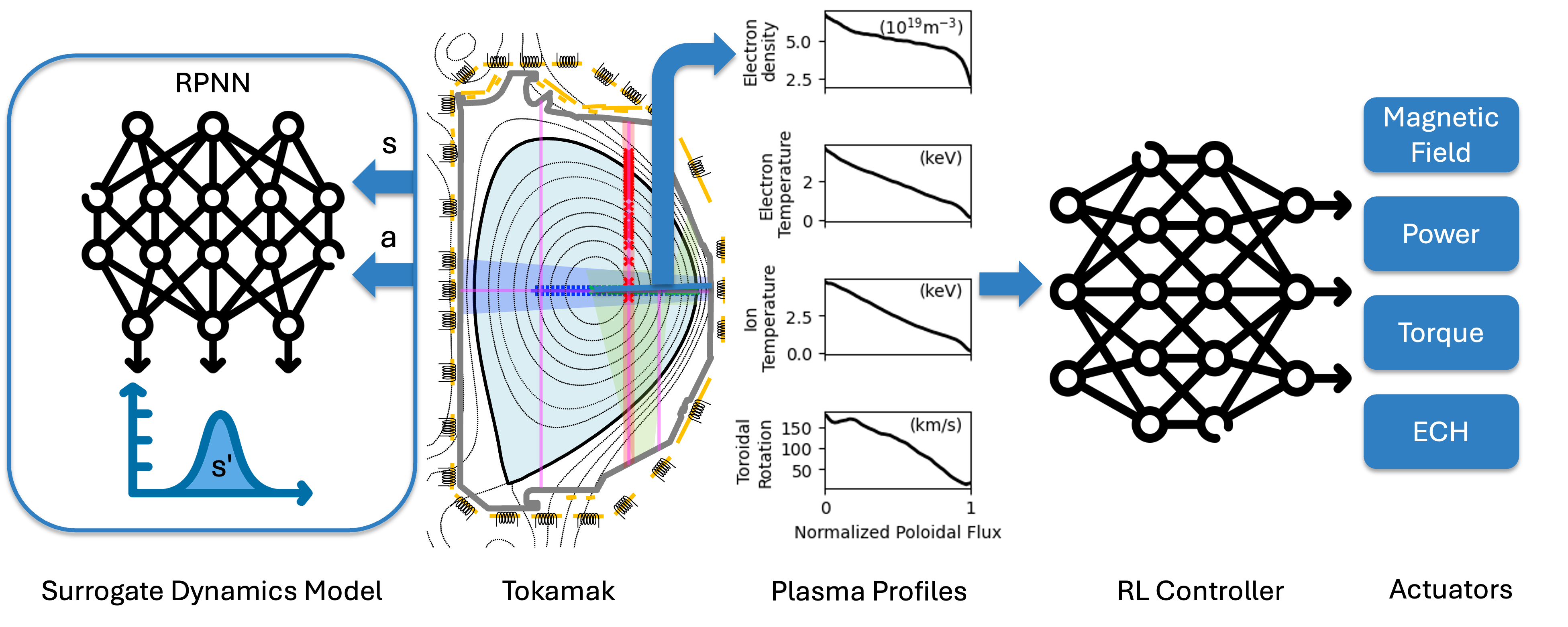
<p>Gaussian noise on MuJoCo is a convenient stress test, but it’s still synthetic. To find out whether any of this matters outside a benchmark, we went looking for a control problem where the “noise” isn’t something we inject — it’s baked into the physics.</p>

<p><img src="/images/rombrl-tokamak.png" alt="ROMBRL applied to Tokamak plasma control" style="width:100%; max-width:650px; display:block; margin:1.5em auto;" /></p>
<p style="text-align:center; font-size:0.9em; margin-top:-1em;"><em>An RL controller trained on a surrogate dynamics model drives plasma profiles toward a target using actuators such as power, torque, and ECH.</em></p>

<p>Tokamak plasma control was a natural fit: confining and shaping a superheated plasma is a genuinely stochastic process. We evaluated on tracking tasks (ion rotation, electron density, and $\beta_N$, a key economic indicator for fusion efficiency) built on an ensemble of recurrent dynamics models calibrated to real operational data from DIII-D, a working tokamak in San Diego.</p>

<p>This benchmark is considerably less forgiving than D4RL MuJoCo — several strong model-based baselines (RAMBO, MOBILE, and a Bayes-adaptive MCTS baseline, BAMCTS) that look competitive on MuJoCo degrade sharply once the dynamics get genuinely messy:</p>

<table>
  <thead>
    <tr>
      <th>Tracking Target</th>
      <th>ROMBRL (ours)</th>
      <th>CQL</th>
      <th>EDAC</th>
      <th>COMBO</th>
      <th>RAMBO</th>
      <th>MOBILE</th>
      <th>BAMCTS</th>
    </tr>
  </thead>
  <tbody>
    <tr>
      <td>$\beta_N$</td>
      <td>**-70.9*** (0.9)</td>
      <td>-78.4 (3.1)</td>
      <td>-63.4 (1.7)</td>
      <td>-84.3 (7.6)</td>
      <td>-121.1 (19.9)</td>
      <td>-133.9 (10.1)</td>
      <td>-111.3 (24.3)</td>
    </tr>
    <tr>
      <td>Density</td>
      <td>**-60.0** (1.9)</td>
      <td>-87.3 (12.5)</td>
      <td>-112.5 (11.1)</td>
      <td>-67.0* (3.1)</td>
      <td>-81.3 (15.7)</td>
      <td>-75.3 (4.3)</td>
      <td>-79.6 (13.8)</td>
    </tr>
    <tr>
      <td>Rotation</td>
      <td>**-10.6** (3.7)</td>
      <td>-39.2* (10.1)</td>
      <td>-95.4 (64.3)</td>
      <td>-69.6 (25.9)</td>
      <td>-300.3 (260.5)</td>
      <td>-257.6 (153.7)</td>
      <td>-305.6 (242.6)</td>
    </tr>
    <tr>
      <td>Average Return</td>
      <td>**-47.1** (1.2)</td>
      <td>-68.3* (6.8)</td>
      <td>-90.4 (11.5)</td>
      <td>-73.6 (5.8)</td>
      <td>-167.6 (91.6)</td>
      <td>-155.5 (47.7)</td>
      <td>-165.5 (84.5)</td>
    </tr>
    <tr>
      <td>Cohen’s *d* vs. ROMBRL</td>
      <td>–</td>
      <td>4.3</td>
      <td>5.3</td>
      <td>6.3</td>
      <td>1.9</td>
      <td>3.2</td>
      <td>2.0</td>
    </tr>
  </tbody>
</table>

<p><em>(negative tracking error, higher/less-negative is better; * marks the second-best result for each row)</em></p>

<p>ROMBRL ranked first on 2 of the 3 tracking targets, second on the third, and had by far the lowest variance across seeds of any method we tested. That gap is the clearest evidence we have that adversarial world-model adaptation isn’t just a MuJoCo party trick — it transfers to the kind of high-stakes, physically-grounded control problem where robustness actually matters.</p>

<h2 id="full-results">Full Results</h2>

<p><strong>D4RL MuJoCo, under 5% measurement noise at deployment.</strong> ROMBRL ranks first on 7/12 tasks and second on 4, with the best average score by a wide margin (Cohen’s <em>d</em> ≥ 2 over every baseline indicates a large, statistically significant effect):</p>

<table>
  <thead>
    <tr>
      <th>Method</th>
      <th>ROMBRL (ours)</th>
      <th>CQL</th>
      <th>EDAC</th>
      <th>COMBO</th>
      <th>RAMBO</th>
      <th>MOBILE</th>
      <th>RORL</th>
      <th>TRACER</th>
      <th>RFQI</th>
    </tr>
  </thead>
  <tbody>
    <tr>
      <td>Average Score</td>
      <td>**77.7** (0.5)</td>
      <td>60.7 (1.2)</td>
      <td>53.7 (4.6)</td>
      <td>55.5 (3.6)</td>
      <td>55.8 (1.3)</td>
      <td>70.7 (2.4)</td>
      <td>62.3 (0.2)</td>
      <td>44.1 (4.8)</td>
      <td>30.9 (2.1)</td>
    </tr>
    <tr>
      <td>Cohen’s *d* vs. ROMBRL</td>
      <td>–</td>
      <td>18.9</td>
      <td>7.4</td>
      <td>8.5</td>
      <td>22.9</td>
      <td>4.1</td>
      <td>40.4</td>
      <td>9.8</td>
      <td>30.7</td>
    </tr>
  </tbody>
</table>

<p><strong>Robustness vs. clean-environment trade-off</strong> (OfflineRL-Kit protocol). ROMBRL matches the best clean-environment performance in the field while losing almost nothing once noise is introduced — where every other baseline gives up 11–27% of its performance:</p>

<table>
  <thead>
    <tr>
      <th>Metric</th>
      <th>ROMBRL (ours)</th>
      <th>CQL</th>
      <th>EDAC</th>
      <th>COMBO</th>
      <th>RAMBO</th>
      <th>MOBILE</th>
      <th>RORL</th>
    </tr>
  </thead>
  <tbody>
    <tr>
      <td>Standard env.</td>
      <td>92.8</td>
      <td>80.4</td>
      <td>93.0</td>
      <td>89.3</td>
      <td>82.7</td>
      <td>**95.9**</td>
      <td>89.5</td>
    </tr>
    <tr>
      <td>Noisy env.</td>
      <td>**93.4**</td>
      <td>77.5</td>
      <td>68.3</td>
      <td>72.2</td>
      <td>66.0</td>
      <td>85.3</td>
      <td>78.7</td>
    </tr>
    <tr>
      <td>Performance drop ↓</td>
      <td>**-0.6%**</td>
      <td>3.6%</td>
      <td>26.6%</td>
      <td>19.1%</td>
      <td>20.2%</td>
      <td>11.1%</td>
      <td>12.1%</td>
    </tr>
  </tbody>
</table>

<p><strong>RWRL-style deployment perturbations</strong> (dropped/stuck observations, body mass, friction, joint damping — applied only at evaluation, trained on clean <code class="language-plaintext highlighter-rouge">hc-med-rep</code> data). ROMBRL achieves the best score on every one of the 5 perturbation types and the smallest overall performance drop, beating dedicated robust baselines RORL and RFQI by a wide margin:</p>

<table>
  <thead>
    <tr>
      <th>Metric</th>
      <th>ROMBRL (ours)</th>
      <th>CQL</th>
      <th>MOBILE</th>
      <th>RAMBO</th>
      <th>RORL</th>
      <th>TRACER</th>
      <th>RFQI</th>
    </tr>
  </thead>
  <tbody>
    <tr>
      <td>Average score under perturbation</td>
      <td>**51.9** (1.0)</td>
      <td>31.2 (1.0)</td>
      <td>45.7 (1.9)</td>
      <td>46.2 (0.2)</td>
      <td>39.3 (1.8)</td>
      <td>23.4 (1.6)</td>
      <td>16.3 (1.6)</td>
    </tr>
    <tr>
      <td>Performance drop ↓</td>
      <td>**25.4%**</td>
      <td>33.2%</td>
      <td>31.6%</td>
      <td>30.0%</td>
      <td>37.6%</td>
      <td>36.2%</td>
      <td>52.1%</td>
    </tr>
  </tbody>
</table>

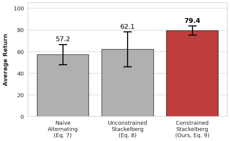
<p><strong>Ablation.</strong> Our full constrained Stackelberg update substantially outperforms both a naive alternating update (à la RAMBO) and an unconstrained Stackelberg update on <code class="language-plaintext highlighter-rouge">walker2d-medium</code>:</p>

<p><img src="/images/rombrl-fig3-ablation.png" alt="Ablation of Stackelberg gradient update mechanisms" style="width:100%; max-width:480px; display:block; margin:1.5em auto;" /></p>
<p style="text-align:center; font-size:0.9em; margin-top:-1em;"><em>Robustness comes specifically from anticipating how the uncertainty-set boundary (via the dual variable λ) shifts with the policy — not just from anticipating the model itself.</em></p>

<h2 id="citation">Citation</h2>

<p>The official PMLR proceedings for ICML 2026 (volume 306) have not been posted yet, so please cite the arXiv version for now — we’ll update this with the final proceedings entry once it’s available:</p>

<div class="language-bibtex highlighter-rouge"><div class="highlight"><pre class="highlight"><code><span class="nc">@article</span><span class="p">{</span><span class="nl">chen2025rombrl</span><span class="p">,</span>
  <span class="na">title</span>   <span class="p">=</span> <span class="s">{Policy-Driven World Model Adaptation for Robust Offline Model-based Reinforcement Learning}</span><span class="p">,</span>
  <span class="na">author</span>  <span class="p">=</span> <span class="s">{Chen, Jiayu and Xu, Le and Venugopal, Aravind and Schneider, Jeff}</span><span class="p">,</span>
  <span class="na">journal</span> <span class="p">=</span> <span class="s">{arXiv preprint arXiv:2505.13709}</span><span class="p">,</span>
  <span class="na">year</span>    <span class="p">=</span> <span class="s">{2025}</span>
<span class="p">}</span>
</code></pre></div></div>

<h2 id="acknowledgements">Acknowledgements</h2>

<p>This work was funded in part by the Department of Energy Fusion Energy Sciences under grant DE-SC0024544.</p>]]></content><author><name>Le Xu</name></author><category term="publication" /><category term="offline-rl" /><category term="robustness" /><category term="model-based-rl" /><summary type="html"><![CDATA[Our paper, “Policy-Driven World Model Adaptation for Robust Offline Model-based Reinforcement Learning”, was presented as a poster at ICML 2026 in Seoul, South Korea. This is joint work between the Agentic Intelligence Lab at the University of Hong Kong, Tsinghua University, and the Robotics Institute at Carnegie Mellon University.]]></summary><media:thumbnail xmlns:media="http://search.yahoo.com/mrss/" url="/preview/pr-10/images/rombrl-cover.png" /><media:content medium="image" url="/preview/pr-10/images/rombrl-cover.png" xmlns:media="http://search.yahoo.com/mrss/" /></entry><entry><title type="html">SAIL-RevKL: Stable and Provable Self-Improving Online LLM Alignment (UAI 2026)</title><link href="/preview/pr-10/2026/08/04/sail-revkl-post.html" rel="alternate" type="text/html" title="SAIL-RevKL: Stable and Provable Self-Improving Online LLM Alignment (UAI 2026)" /><published>2026-08-04T00:00:00+00:00</published><updated>2026-10-10T14:58:01+00:00</updated><id>/preview/pr-10/2026/08/04/sail-revkl-post</id><content type="html" xml:base="/preview/pr-10/2026/08/04/sail-revkl-post.html"><![CDATA[<p>Our paper, <strong>“On the Convergence of Self-Improving Online LLM Alignment,”</strong> appeared at the <strong>42nd Conference on Uncertainty in Artificial Intelligence (UAI 2026)</strong>. It addresses a basic theoretical gap behind self-improving alignment.</p>

<h2 id="research-question">Research Question</h2>

<p><strong>Can we establish a global convergence guarantee for online RLHF formulated as a bilevel optimization problem?</strong></p>

<p><a href="https://proceedings.mlr.press/v337/wu26c.html"><strong>Proceedings</strong></a> · <a href="https://arxiv.org/abs/2606.31524"><strong>arXiv</strong></a> · <a href="/images/sail-revkl-poster.png"><strong>Poster</strong></a> · <a href="https://github.com/xudongwu-0/SAIL_mujoco"><strong>MuJoCo Code</strong></a> · <a href="https://github.com/xudongwu-0/SAIL_LLM">** Code**</a></p>

<figure class="figure">
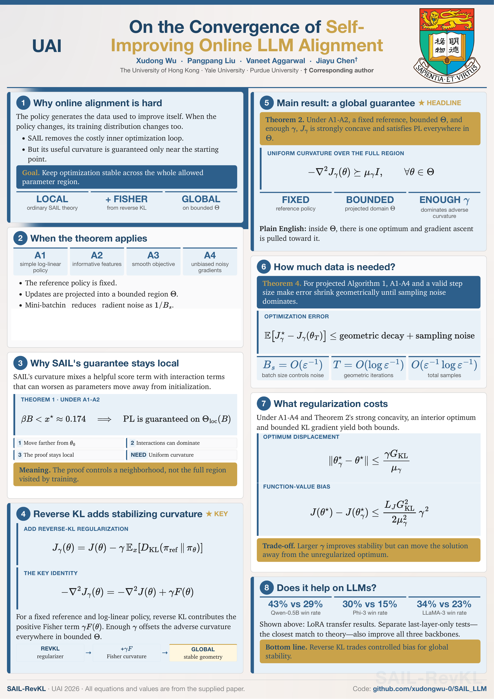
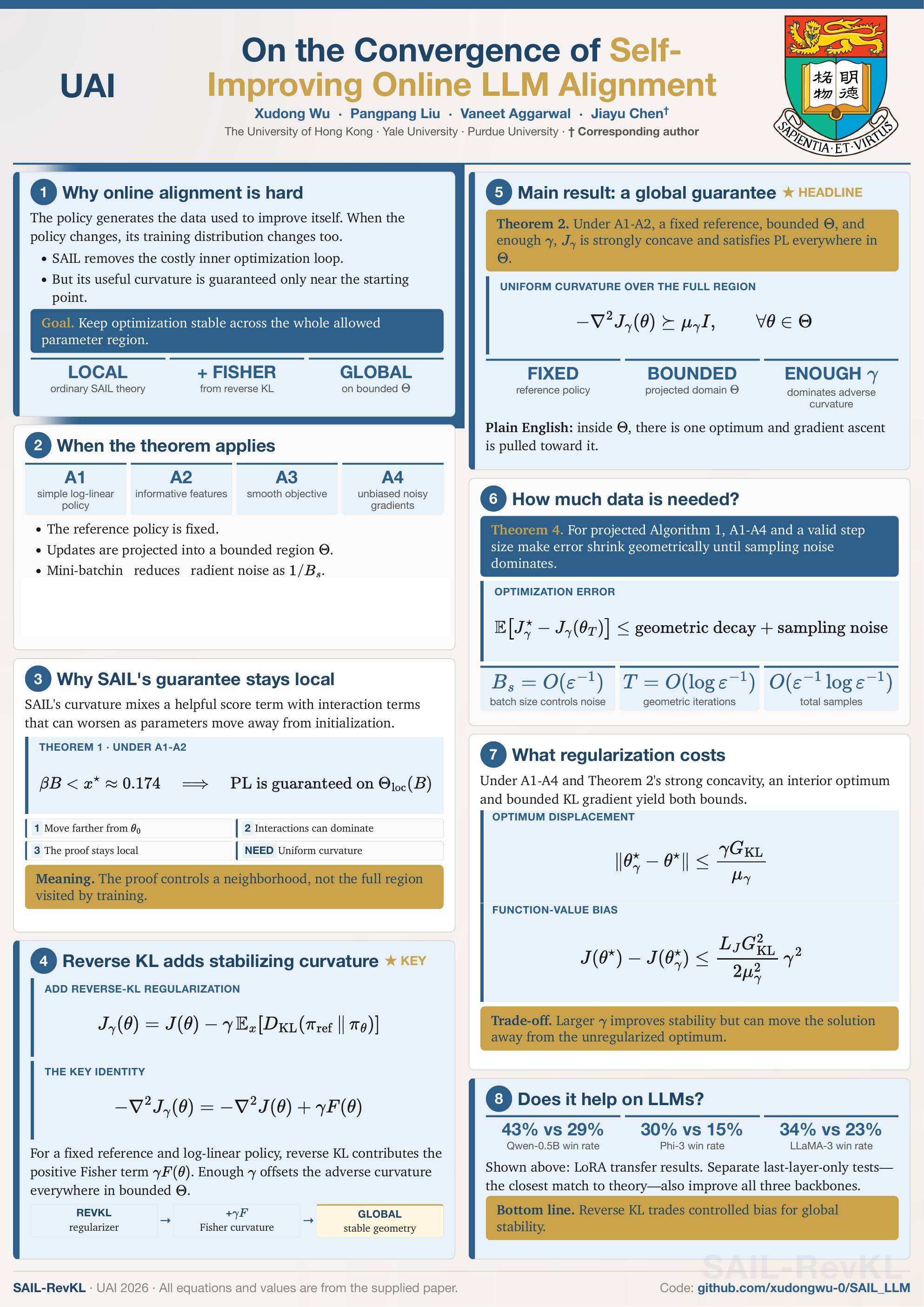
  <a href="/preview/pr-10/images/sail-revkl-poster.png" class="figure-image" aria-label="Our UAI 2026 poster. Click the image to open it at full resolution.">
    <img src="/preview/pr-10/images/sail-revkl-poster.png" style="
        width: 100%;
        max-height: unset;
      " alt="Our UAI 2026 poster. Click the image to open it at full resolution." loading="lazy" onerror="this.src = '/preview/pr-10/images/fallback.svg'; this.onerror = null;" />
  </a>
  
    <figcaption class="figure-caption">
      Our UAI 2026 poster. Click the image to open it at full resolution.

    </figcaption>
  
</figure>

<h2 id="tldr">TL;DR</h2>

<p>Our answer is conditional but positive. We first show that the original <strong>Self-Improving Alignment (SAIL)</strong> objective is guaranteed to have favorable curvature only near its initialization. We then introduce <strong>SAIL-RevKL</strong>, which adds</p>

<p>$$
\gamma\,\mathbb{E}_x!\left[
D_{\mathrm{KL}}!\left(
\pi_{\mathrm{ref}}(\cdot\mid x)\,\Vert\,\pi_\theta(\cdot\mid x)
\right)
\right]
$$</p>

<p>as a penalty. For a fixed reference and a log-linear policy, the Hessian of this reverse KL is the Fisher information matrix. With enough regularization, that positive curvature dominates the adverse curvature of SAIL throughout the full bounded parameter region. This yields global strong concavity and a Polyak-Lojasiewicz (PL) condition for the regularized surrogate, together with near-linear dependence on the inverse target accuracy.</p>

<h2 id="why-bilevel-formulated-online-rlhf-is-hard">Why Bilevel-Formulated Online RLHF Is Hard</h2>

<p>Offline preference optimization trains on a fixed dataset. Online RLHF instead couples two learning problems: a reward model is fitted from preferences over responses generated by the current policy, and the policy is updated against that learned reward. This interaction is naturally formulated as a bilevel optimization problem because the solution of one level determines the objective and data distribution of the other.</p>

<p>SAIL uses the reward-policy equivalence to reduce this computationally expensive bilevel problem to an efficient single-level surrogate. If $\mathcal{D}_\theta$ denotes the policy-dependent response and preference distribution, that surrogate has the form</p>

<p>$$
J(\theta)
=
\mathbb{E}_{(x,y_w,y_l)\sim\mathcal{D}_\theta}
!\left[
\log\sigma!\left(
\beta\log\frac{\pi_\theta(y_w\mid x)}{\pi_{\mathrm{SFT}}(y_w\mid x)}
-
\beta\log\frac{\pi_\theta(y_l\mid x)}{\pi_{\mathrm{SFT}}(y_l\mid x)}
\right)
\right].
$$</p>

<p>This dependence matters. Standard performance-difference arguments assume that the reward or evaluation measure is independent of the policy appearing inside the advantage. That assumption no longer holds here, so convergence cannot be inherited directly from ordinary policy-gradient analysis. We instead analyze the geometry of $J$ itself.</p>

<p>The negative Hessian of $J$ decomposes into four terms. Some are stabilizing, while interaction terms can become unfavorable as $\theta$ moves away from the initial SFT parameters $\theta_0$. The proof must therefore control the objective’s curvature throughout the region the algorithm may visit, not only at its starting point.</p>

<div class="alert" style="--color: #0ea5e9">
  
  <i class="icon fa-solid fa-circle-info"></i>
  <div class="alert-content">
    <p><strong>Hint: why the research question is hard.</strong> In this bilevel formulation of online RLHF, the reward-learning level depends on data from the current policy, while the policy-update level depends on the learned reward. The two levels therefore evolve together, so a fixed-data convergence argument does not directly apply.</p>

  </div>
</div>

<h2 id="assumptions-and-scope">Assumptions and Scope</h2>

<p>The global theorem is explicit about its scope. It applies to the following setting:</p>

<table>
  <thead>
    <tr>
      <th>Assumption</th>
      <th>Mathematical condition</th>
      <th>Role in the analysis</th>
    </tr>
  </thead>
  <tbody>
    <tr>
      <td>**A1: Log-linear policy**</td>
      <td>$\pi_\theta(a\mid s)\propto\exp(\theta^\top\psi(s,a))$, with $\max_{s,a}\Vert\psi(s,a)\Vert_2\le 1$ and $\Vert\theta-\theta_0\Vert_2\le B_\theta$</td>
      <td>Makes the objective’s curvature analyzable on a bounded parameter set.</td>
    </tr>
    <tr>
      <td>**A2: Informative features**</td>
      <td>$F_\rho(\theta)\succeq\mu_F I$ uniformly over the feasible set</td>
      <td>Ensures the Fisher curvature is positive in every parameter direction.</td>
    </tr>
    <tr>
      <td>**A3: Smooth objective**</td>
      <td>$J_\gamma$ is $L$-smooth</td>
      <td>Controls the change of the gradient and permits a stable stepsize.</td>
    </tr>
    <tr>
      <td>**A4: Stochastic gradients**</td>
      <td>Each sample gradient is unbiased and has variance at most $\sigma_g^2$</td>
      <td>Makes the mini-batch noise decay as $\sigma_g^2/B_s$.</td>
    </tr>
  </tbody>
</table>

<p>Two construction choices are also essential. The reference policy $\pi_{\mathrm{ref}}$ is fixed during the analyzed update, and projected gradient ascent keeps every iterate inside $\Theta$, the radius-$B_\theta$ Euclidean ball centered at $\theta_0$.</p>

<p><strong>Scope of the result.</strong> The word “global” below means global <strong>within this full bounded feasible set</strong>. The LoRA experiments test whether the method remains useful beyond these assumptions; the last-layer-only experiments are the closest empirical match to A1.</p>

<h2 id="core-theorem-global-convergence-of-sail-revkl">Core Theorem: Global Convergence of SAIL-RevKL</h2>

<p>The original SAIL surrogate is guaranteed to have favorable geometry only near its initialization. We add a reverse-KL penalty and optimize</p>

<p>$$
J_\gamma(\theta)
=
J(\theta)
-
\gamma\,\mathbb{E}_x!\left[
D_{\mathrm{KL}}!\left(
\pi_{\mathrm{ref}}(\cdot\mid x)\,\Vert\,\pi_\theta(\cdot\mid x)
\right)
\right].
$$</p>

<p>For a fixed reference and a log-linear policy, the reverse-KL Hessian is the Fisher information matrix, so</p>

<p>$$
-\nabla^2J_\gamma(\theta)
=
-\nabla^2J(\theta)+\gamma F(\theta).
$$</p>

<h3 id="theorem-global-convergence-on-the-feasible-set">Theorem (Global convergence on the feasible set)</h3>

<p>Let $\Theta$ be the radius-$B_\theta$ Euclidean ball centered at $\theta_0$. Suppose A1-A4 hold, $\pi_{\mathrm{ref}}$ remains fixed during optimization, and projected updates keep every iterate in $\Theta$. Choose $\gamma$ sufficiently large to satisfy the explicit curvature threshold in Theorem 2 of the paper, so that the Fisher term dominates the adverse curvature of the original SAIL objective throughout $\Theta$.</p>

<p>Then $J_\gamma$ is $\mu$-strongly concave on all of $\Theta$ and satisfies the PL inequality</p>

<p>$$
\Vert\nabla J_\gamma(\theta)\Vert_2^2
\ge
2\mu\left(J_\gamma(\theta_\gamma^{\ast})-J_\gamma(\theta)\right),
\qquad \theta\in\Theta,
$$</p>

<p>where $\theta_\gamma^{\ast}=\arg\max_{\theta\in\Theta}J_\gamma(\theta)$ is the unique maximizer. Moreover, for projected mini-batch stochastic gradient ascent with a valid constant stepsize, there exist constants $q\in(0,1)$ and $C&gt;0$ such that</p>

<p>$$
\mathbb{E}!\left[
J_\gamma(\theta_\gamma^{\ast})-J_\gamma(\theta_T)
\right]
\le
q^T\left(J_\gamma(\theta_\gamma^{\ast})-J_\gamma(\theta_0)\right)
+
\frac{C\sigma_g^2}{B_s}.
$$</p>

<p>Thus the optimization error decreases geometrically until it reaches the mini-batch noise floor. Taking $B_s=\widetilde{\mathcal{O}}(\varepsilon^{-1})$ and $T=\widetilde{\mathcal{O}}(\log\varepsilon^{-1})$ gives an $\varepsilon$ expected function-value gap with total sample complexity</p>

<p>$$
\widetilde{\mathcal{O}}!\left(
\varepsilon^{-1}\log\varepsilon^{-1}
\right).
$$</p>

<div class="alert" style="--color: #0ea5e9">
  
  <i class="icon fa-solid fa-circle-info"></i>
  <div class="alert-content">
    <p><strong>Hint: what the theorem answers.</strong> For the SAIL reduction of bilevel-formulated online RLHF, reverse KL turns a local convergence certificate into a global, non-asymptotic guarantee over the entire bounded feasible set.</p>

  </div>
</div>

<p>The theorem is proved in a deliberately controlled log-linear setting. We next test whether the same regularized objective is useful when training real language models.</p>

<h2 id="llm-alignment-results">LLM Alignment Results</h2>

<p>The main experiments use LoRA fine-tuning and GPT-4 as an LLM judge. PKU-SafeRLHF evaluates the balance between helpfulness and harmlessness, while UltraFeedback focuses on general instruction following. Pairwise win rate is the primary comparison below; tie rate and mean GPT score difference are reported separately because they capture different aspects of the judge outcomes.</p>

<p><strong>PKU-SafeRLHF, Qwen 0.5B</strong></p>

<table>
  <thead>
    <tr>
      <th>Method</th>
      <th style="text-align: right">Pairwise win rate</th>
      <th style="text-align: right">Tie rate</th>
      <th style="text-align: right">Mean GPT score difference</th>
    </tr>
  </thead>
  <tbody>
    <tr>
      <td>DPO</td>
      <td style="text-align: right">26.0%</td>
      <td style="text-align: right">14.0%</td>
      <td style="text-align: right">-2.209</td>
    </tr>
    <tr>
      <td>SAIL</td>
      <td style="text-align: right">29.0%</td>
      <td style="text-align: right">0.0%</td>
      <td style="text-align: right">-2.004</td>
    </tr>
    <tr>
      <td>**SAIL-RevKL**</td>
      <td style="text-align: right">**43.0%**</td>
      <td style="text-align: right">6.0%</td>
      <td style="text-align: right">**-0.885**</td>
    </tr>
  </tbody>
</table>

<p><strong>UltraFeedback</strong></p>

<table>
  <thead>
    <tr>
      <th>Backbone</th>
      <th>Method</th>
      <th style="text-align: right">Pairwise win rate</th>
      <th style="text-align: right">Tie rate</th>
      <th style="text-align: right">Mean GPT score difference</th>
    </tr>
  </thead>
  <tbody>
    <tr>
      <td>Qwen 0.5B</td>
      <td>DPO</td>
      <td style="text-align: right">0.0%</td>
      <td style="text-align: right">7.0%</td>
      <td style="text-align: right">-2.580</td>
    </tr>
    <tr>
      <td>Qwen 0.5B</td>
      <td>SAIL</td>
      <td style="text-align: right">1.0%</td>
      <td style="text-align: right">8.0%</td>
      <td style="text-align: right">-2.110</td>
    </tr>
    <tr>
      <td>Qwen 0.5B</td>
      <td>**SAIL-RevKL**</td>
      <td style="text-align: right">**3.0%**</td>
      <td style="text-align: right">**18.0%**</td>
      <td style="text-align: right">**-1.300**</td>
    </tr>
    <tr>
      <td>Phi-3 3.8B</td>
      <td>DPO</td>
      <td style="text-align: right">11.0%</td>
      <td style="text-align: right">15.0%</td>
      <td style="text-align: right">-1.160</td>
    </tr>
    <tr>
      <td>Phi-3 3.8B</td>
      <td>SAIL</td>
      <td style="text-align: right">15.0%</td>
      <td style="text-align: right">**60.0%**</td>
      <td style="text-align: right">**-0.150**</td>
    </tr>
    <tr>
      <td>Phi-3 3.8B</td>
      <td>**SAIL-RevKL**</td>
      <td style="text-align: right">**30.0%**</td>
      <td style="text-align: right">40.0%</td>
      <td style="text-align: right">-0.300</td>
    </tr>
    <tr>
      <td>LLaMA-3 8B</td>
      <td>DPO</td>
      <td style="text-align: right">22.0%</td>
      <td style="text-align: right">24.0%</td>
      <td style="text-align: right">-0.930</td>
    </tr>
    <tr>
      <td>LLaMA-3 8B</td>
      <td>SAIL</td>
      <td style="text-align: right">23.0%</td>
      <td style="text-align: right">**29.0%**</td>
      <td style="text-align: right">-0.700</td>
    </tr>
    <tr>
      <td>LLaMA-3 8B</td>
      <td>**SAIL-RevKL**</td>
      <td style="text-align: right">**34.0%**</td>
      <td style="text-align: right">**29.0%**</td>
      <td style="text-align: right">**-0.230**</td>
    </tr>
  </tbody>
</table>

<p>The headline comparison is the pairwise win rate against vanilla SAIL: <strong>43% vs. 29%</strong> on Qwen with PKU-SafeRLHF, <strong>30% vs. 15%</strong> on Phi-3 with UltraFeedback, and <strong>34% vs. 23%</strong> on LLaMA-3 with UltraFeedback.</p>

<h3 id="a-theory-aligned-test">A theory-aligned test</h3>

<p>LoRA changes nonlinear features and is not a direct instantiation of the log-linear policy in A1. We therefore also freeze each backbone and train only its final linear layer on UltraFeedback U10. This isolates the regime that most closely matches the theory.</p>

<table>
  <thead>
    <tr>
      <th>Backbone</th>
      <th>Method</th>
      <th style="text-align: right">$\gamma$</th>
      <th style="text-align: right">Win rate</th>
      <th style="text-align: right">Lose rate</th>
      <th style="text-align: right">Tie rate</th>
    </tr>
  </thead>
  <tbody>
    <tr>
      <td>Qwen 0.5B</td>
      <td>DPO</td>
      <td style="text-align: right">-</td>
      <td style="text-align: right">1.0%</td>
      <td style="text-align: right">91.0%</td>
      <td style="text-align: right">8.0%</td>
    </tr>
    <tr>
      <td>Qwen 0.5B</td>
      <td>SAIL</td>
      <td style="text-align: right">-</td>
      <td style="text-align: right">1.0%</td>
      <td style="text-align: right">93.0%</td>
      <td style="text-align: right">6.0%</td>
    </tr>
    <tr>
      <td>Qwen 0.5B</td>
      <td>SAIL-RevKL</td>
      <td style="text-align: right">$10^{-3}$</td>
      <td style="text-align: right">3.0%</td>
      <td style="text-align: right">91.0%</td>
      <td style="text-align: right">6.0%</td>
    </tr>
    <tr>
      <td>Qwen 0.5B</td>
      <td>**SAIL-RevKL**</td>
      <td style="text-align: right">$10^{-2}$</td>
      <td style="text-align: right">**4.0%**</td>
      <td style="text-align: right">86.0%</td>
      <td style="text-align: right">10.0%</td>
    </tr>
    <tr>
      <td>Qwen 0.5B</td>
      <td>SAIL-RevKL</td>
      <td style="text-align: right">$10^{-1}$</td>
      <td style="text-align: right">3.0%</td>
      <td style="text-align: right">**83.0%**</td>
      <td style="text-align: right">**14.0%**</td>
    </tr>
    <tr>
      <td>Phi-3 3.8B</td>
      <td>DPO</td>
      <td style="text-align: right">-</td>
      <td style="text-align: right">13.0%</td>
      <td style="text-align: right">**37.0%**</td>
      <td style="text-align: right">**50.0%**</td>
    </tr>
    <tr>
      <td>Phi-3 3.8B</td>
      <td>SAIL</td>
      <td style="text-align: right">-</td>
      <td style="text-align: right">16.0%</td>
      <td style="text-align: right">40.0%</td>
      <td style="text-align: right">44.0%</td>
    </tr>
    <tr>
      <td>Phi-3 3.8B</td>
      <td>SAIL-RevKL</td>
      <td style="text-align: right">$10^{-3}$</td>
      <td style="text-align: right">16.0%</td>
      <td style="text-align: right">40.0%</td>
      <td style="text-align: right">44.0%</td>
    </tr>
    <tr>
      <td>Phi-3 3.8B</td>
      <td>SAIL-RevKL</td>
      <td style="text-align: right">$10^{-2}$</td>
      <td style="text-align: right">21.0%</td>
      <td style="text-align: right">43.0%</td>
      <td style="text-align: right">36.0%</td>
    </tr>
    <tr>
      <td>Phi-3 3.8B</td>
      <td>**SAIL-RevKL**</td>
      <td style="text-align: right">$10^{-1}$</td>
      <td style="text-align: right">**23.0%**</td>
      <td style="text-align: right">43.0%</td>
      <td style="text-align: right">34.0%</td>
    </tr>
    <tr>
      <td>LLaMA-3 8B</td>
      <td>DPO</td>
      <td style="text-align: right">-</td>
      <td style="text-align: right">0.0%</td>
      <td style="text-align: right">93.0%</td>
      <td style="text-align: right">7.0%</td>
    </tr>
    <tr>
      <td>LLaMA-3 8B</td>
      <td>SAIL</td>
      <td style="text-align: right">-</td>
      <td style="text-align: right">5.0%</td>
      <td style="text-align: right">69.0%</td>
      <td style="text-align: right">26.0%</td>
    </tr>
    <tr>
      <td>LLaMA-3 8B</td>
      <td>SAIL-RevKL</td>
      <td style="text-align: right">$10^{-3}$</td>
      <td style="text-align: right">7.0%</td>
      <td style="text-align: right">67.0%</td>
      <td style="text-align: right">26.0%</td>
    </tr>
    <tr>
      <td>LLaMA-3 8B</td>
      <td>SAIL-RevKL</td>
      <td style="text-align: right">$10^{-2}$</td>
      <td style="text-align: right">7.0%</td>
      <td style="text-align: right">**58.0%**</td>
      <td style="text-align: right">**35.0%**</td>
    </tr>
    <tr>
      <td>LLaMA-3 8B</td>
      <td>**SAIL-RevKL**</td>
      <td style="text-align: right">$10^{-1}$</td>
      <td style="text-align: right">**13.0%**</td>
      <td style="text-align: right">59.0%</td>
      <td style="text-align: right">28.0%</td>
    </tr>
  </tbody>
</table>

<p>SAIL-RevKL improves the best win rate over vanilla SAIL on all three backbones. The preferred coefficient is scale-dependent: $10^{-2}$ for Qwen 0.5B and $10^{-1}$ for Phi-3 3.8B and LLaMA-3 8B. This is consistent with the theory’s curvature-bias trade-off and shows why $\gamma$ should be tuned rather than treated as a universal constant.</p>

<div class="alert" style="--color: #0ea5e9">
  
  <i class="icon fa-solid fa-circle-info"></i>
  <div class="alert-content">
    <p><strong>Hint: how to read the evidence.</strong> The LoRA results show that SAIL-RevKL improves pairwise win rates beyond the policy class covered by the theorem, but they do not prove global convergence for LoRA. Frozen-last-layer training is the closer empirical check of the log-linear regime.</p>

  </div>
</div>

<h2 id="citation">Citation</h2>

<div class="language-bibtex highlighter-rouge"><div class="highlight"><pre class="highlight"><code><span class="nc">@inproceedings</span><span class="p">{</span><span class="nl">wu2026convergence</span><span class="p">,</span>
  <span class="na">title</span>     <span class="p">=</span> <span class="s">{On the Convergence of Self-Improving Online {LLM} Alignment}</span><span class="p">,</span>
  <span class="na">author</span>    <span class="p">=</span> <span class="s">{Wu, Xudong and Liu, Pangpang and Aggarwal, Vaneet and Chen, Jiayu}</span><span class="p">,</span>
  <span class="na">booktitle</span> <span class="p">=</span> <span class="s">{Proceedings of the 42nd Conference on Uncertainty in Artificial Intelligence}</span><span class="p">,</span>
  <span class="na">pages</span>     <span class="p">=</span> <span class="s">{7433--7467}</span><span class="p">,</span>
  <span class="na">year</span>      <span class="p">=</span> <span class="s">{2026}</span><span class="p">,</span>
  <span class="na">volume</span>    <span class="p">=</span> <span class="s">{337}</span><span class="p">,</span>
  <span class="na">series</span>    <span class="p">=</span> <span class="s">{Proceedings of Machine Learning Research}</span>
<span class="p">}</span>
</code></pre></div></div>

<h2 id="acknowledgements">Acknowledgements</h2>

<p>This work was supported in part by the Seed Fund for PI Research, Basic Research, from The University of Hong Kong under Project Code 2502251784.</p>]]></content><author><name>Xudong Wu</name></author><category term="publication" /><category term="llm-alignment" /><category term="optimization" /><category term="theory" /><summary type="html"><![CDATA[Our paper, “On the Convergence of Self-Improving Online LLM Alignment,” appeared at the 42nd Conference on Uncertainty in Artificial Intelligence (UAI 2026). It addresses a basic theoretical gap behind self-improving alignment.]]></summary><media:thumbnail xmlns:media="http://search.yahoo.com/mrss/" url="/preview/pr-10/images/logo.png" /><media:content medium="image" url="/preview/pr-10/images/logo.png" xmlns:media="http://search.yahoo.com/mrss/" /></entry><entry><title type="html">Verlog - A Multi-turn RL framework for LLM agents</title><link href="/preview/pr-10/2025/08/15/technical-post.html" rel="alternate" type="text/html" title="Verlog - A Multi-turn RL framework for LLM agents" /><published>2025-08-15T00:00:00+00:00</published><updated>2026-10-10T14:58:01+00:00</updated><id>/preview/pr-10/2025/08/15/technical-post</id><content type="html" xml:base="/preview/pr-10/2025/08/15/technical-post.html"><![CDATA[<div style="display: flex; justify-content: center; align-items: center; flex-wrap: wrap; gap: 24px; width: 100%;">
  <a href="https://github.com/WentseChen/Verlog" target="_blank" style="text-decoration: none; display: flex; align-items: center;">
    <img src="https://cdn.jsdelivr.net/npm/simple-icons@v9/icons/github.svg" alt="GitHub" width="30" height="30" style="vertical-align: middle;" />
    <span style="vertical-align: middle; font-size: 16px; margin-left: 6px;">Source Code</span>
  </a>

  <a href="https://wandb.ai/cwz19/verlog?nw=nwusercwz19" target="_blank" style="text-decoration: none; display: flex; align-items: center;">
    <img src="https://raw.githubusercontent.com/wandb/assets/main/wandb-dots-logo.svg" alt="W&amp;B" width="30" height="30" style="vertical-align: middle;" />
    <span style="vertical-align: middle; font-size: 16px; margin-left: 6px;">Experiment Logs</span>
  </a>
</div>

<p>Verlog is a multi-turn reinforcement learning framework built for <strong>long-horizon LLM-agentic tasks with highly variable episode lengths</strong>. Extending <a href="https://github.com/volcengine/verl">VeRL</a> and <a href="https://github.com/balrog-ai/BALROG">BALROG</a> while following the proven design principles of <a href="https://github.com/ikostrikov/pytorch-a2c-ppo-acktr-gail">pytorch-a2c-ppo-acktr-gail</a>, it introduces specialized optimizations for stable and efficient training when episodes span from short interactions to hundreds of turns. Whereas prior frameworks like <a href="https://github.com/volcengine/verl">VeRL</a> and <a href="https://ragen-ai.github.io">RAGEN</a> effectively handle tasks with ~10 turns, and <a href="https://github.com/langfengQ/verl-agent">verl-agent</a> scales up to 50 turns, Verlog is designed to operate in environments with <strong>over 400 turns</strong>, making it uniquely suited for complex, long-term decision-making. This capability has been validated across challenging domains such as BabyAI, BabaIsAI, and Crafter, where it consistently achieves strong performance out of the box. In Crafter, for instance, episode lengths range from 70 to 400 steps with an average of about 190.</p>

<p>Please kindly check <a href="https://wentsechen.github.io/Verlog_blogpost/">https://wentsechen.github.io/Verlog_blogpost/</a> for details.</p>]]></content><author><name>Wentse Chen</name></author><category term="technique" /><summary type="html"><![CDATA[Source Code]]></summary><media:thumbnail xmlns:media="http://search.yahoo.com/mrss/" url="/preview/pr-10/images/crafter_zeroshot.gif" /><media:content medium="image" url="/preview/pr-10/images/crafter_zeroshot.gif" xmlns:media="http://search.yahoo.com/mrss/" /></entry><entry><title type="html">Available Research Positions at the Agentic Intelligence Lab @ The University of Hong Kong</title><link href="/preview/pr-10/2025/01/03/hiring-post.html" rel="alternate" type="text/html" title="Available Research Positions at the Agentic Intelligence Lab @ The University of Hong Kong" /><published>2025-01-03T00:00:00+00:00</published><updated>2026-10-10T14:58:01+00:00</updated><id>/preview/pr-10/2025/01/03/hiring-post</id><content type="html" xml:base="/preview/pr-10/2025/01/03/hiring-post.html"><![CDATA[<h2 id="about-the-pi">About the PI</h2>

<p>Jiayu Chen (陈佳玉) is an incoming Tenure-Track Assistant Professor at the <a href="https://www.dase.hku.hk/">Department of Data and Systems Engineering, The University of Hong Kong</a>. Currently, he is a Postdoctoral Fellow at the <a href="https://www.cs.cmu.edu/">School of Computer Science, Carnegie Mellon University</a>, working under the supervision of <a href="https://www.cs.cmu.edu/~schneide/">Professor Jeff Schneider</a> on data-driven profile control for nuclear fusion, as part of a joint research program with the <a href="https://control.princeton.edu/">Plasma Control Group, Princeton University</a>.</p>

<p>Dr. Chen earned his Ph.D. in Industrial Engineering and Operations Research from the <a href="https://engineering.purdue.edu/IE">Edwardson School of Industrial Engineering, Purdue University</a> and a Bachelor of Engineering from the <a href="https://www.coe.pku.edu.cn/">College of Engineering, Peking University</a>. During his Ph.D., he was co-advised by <a href="https://engineering.purdue.edu/CLANLabs">Professor Vaneet Aggarwal (Purdue University)</a>, an expert in theoretical reinforcement learning, and <a href="https://www2.seas.gwu.edu/~tlan/">Professor Tian Lan (George Washington University)</a>, an expert in multi-agent systems.</p>

<p>He is the director of the <a href="https://agentic-intelligence-lab.org/">Agentic Intelligence Lab</a>, where his research focuses on Learning for Sequential Decision-Making and Continuous Control. Dr. Chen has published extensively in top venues such as NeurIPS, ICML, ICRA, ICAPS, AAMAS, TMLR, and IEEE TNNLS as the first author. His work has been recognized with prestigious awards, including the Oracle Research Award and the Purdue Research Grant.</p>

<h2 id="about-the-universitydepartment">About the University/Department</h2>

<p>Founded in 1911, the University of Hong Kong (HKU) is the oldest tertiary education institution in Hong Kong, renowned globally for its excellence in teaching, research, and innovation. According to the QS World University Rankings, HKU is currently ranked <strong>2nd in Asia</strong> and <strong>17th worldwide.</strong> Studying at HKU offers unique advantages: its location in the vibrant, internationally connected city of Hong Kong provides unmatched access to global business networks, a multicultural environment, and close proximity to the thriving economies of the Greater Bay Area.</p>

<p>In the midst of the artificial intelligence and big data revolution, the <a href="https://www.dase.hku.hk/about-us/introduction">Department of Data and Systems Engineering (DASE)</a> upholds the philosophy of “computing-in-practice”. The vision is to bridge the cyber and physical worlds by integrating data science methodologies, such as artificial intelligence, with human tools like robots to create greater value for humanity. To achieve this goal, DASE focuses on three key areas: <strong>Data Engineering and Analytics</strong>, <strong>Human-Machine Cooperation</strong>, and <strong>Robotics and Automation</strong>.</p>

<h2 id="research-areas">Research Areas</h2>

<p>The Agentic Intelligence Lab conducts broad research across Machine Learning, Robotics, and Operations Research. At present, our work focuses on advancing the following key areas:</p>

<ul>
  <li>Theoretical foundations, algorithm design, and applications of (Multi-agent) Reinforcement Learning;</li>
  <li>Developing a unified theoretical framework for Reinforcement Learning, Optimal Control, and Stochastic Optimization;</li>
  <li>Scaling Laws in sequential decision-making, with a special emphasis on efficient (Multi-agent) Monte Carlo Tree Search algorithms and advanced Reasoning Models;</li>
  <li>Robotic Foundation Models;</li>
  <li>End-to-end multi-modal learning for Humanoid Robotic Control and its industrial applications;</li>
  <li>Post-training techniques for Large Language Model agents and their applications in sequential decision-making;</li>
  <li>Artificial General Intelligence grounded in the principles of <a href="http://www.incompleteideas.net/Talks/AlbertaPlan.pdf">The Alberta Plan</a>.</li>
</ul>

<h2 id="available-positions">Available Positions</h2>

<p>We have the following openings:</p>

<!-- - **Two fully funded Ph.D. positions** starting in **Fall 2025 (as early as July)**
- Openings for **postdoctoral researchers**, **self-financed Ph.D. students**, **part-time Ph.D. students**, **research assistants**, and **visiting scholars** are available **year-round**  -->

<ul>
  <li><strong>Fully funded Ph.D. positions</strong> starting in <strong>Fall 2025</strong> have been taken.</li>
  <li>Openings for <strong>self-financed Ph.D. students</strong> and  <strong>research assistants</strong> are available <strong>year-round</strong>.</li>
  <li>❗❗❗ We have an available postdoc position in reinforcement learning and robotic learning.</li>
  <li>❗❗❗ We need a <strong>remote research intern</strong> for a project to benchmark offline RL and control methods for plasma control in nuclear fusion. Please check this <a href="https://github.com/LucasCJYSDL/Offline-RL-Kit-for-Nuclear-Fusion">repo</a> for details and reach out to Dr. Jiayu Chen if interested.</li>
</ul>

<p>Ph.D. and postdoctoral applicants are expected to have <strong>strong proficiency in mathematics or programming, along with demonstrated self-motivation and resilience</strong>. Candidates with expertise in the following areas are highly preferred: Humanoid Robots, Large Language/Reasoning Models, Control Theory, Optimization Theory, Statistical Machine Learning.</p>

<p>We offer competitive remuneration. For Ph.D. students, the basic level of scholarship is 18,760 HK dollars per month. For <a href="https://www.hr.hku.hk/career_opportunities/pdf-rap.html">postdocal researchers</a>, the basic salary is no less than 30,000 HK dollars per month. Outstanding candidates are encouraged to apply for the <a href="https://gradsch.hku.hk/prospective_students/fees_scholarships_and_financial_support/hku_presidential_phd_scholar_programme">HKU Presidential PhD Scholar Programme (HKUPS)</a>, <a href="https://gradsch.hku.hk/prospective_students/fees_scholarships_and_financial_support/hong_kong_phd_fellowship_scheme">Hong Kong PhD Fellowship Scheme (HKPFS)</a>, and <a href="https://www.ugc.edu.hk/eng/rgc/funding_opport/pdfs/">RGC Postdoctoral Fellowship Scheme (PDFS)</a> to get financial support of approximately 430,000 HK dollars annaly.</p>

<p>We also provide opportunities for visiting experiences at top U.S. universities such as UC Berkeley, UIUC, CMU, Purdue, and GWU. For <strong>research assistants</strong>, we offer strong recommendation letters and ample opportunities to publish papers in top machine learning and robotics venues.</p>

<p>For detailed requirements and additional information, please refer to the respective categories in <a href="https://agentic-intelligence-lab.org/openings/">openings</a>.  If interested, please contact <a href="https://agentic-intelligence-lab.org/members/jiayu-chen.html">Dr. Jiayu Chen</a> directly through <u>jiayuc@hku.hk</u>. The Ph.D. application system at HKU accepts submissions <strong>year-round</strong>.</p>

<p><u>Deeply sorry that I am unable to respond to every inquiry unless it is to send an interview invitation.</u></p>]]></content><author><name>Jiayu Chen</name></author><category term="hiring" /><summary type="html"><![CDATA[About the PI]]></summary><media:thumbnail xmlns:media="http://search.yahoo.com/mrss/" url="/preview/pr-10/images/logo.png" /><media:content medium="image" url="/preview/pr-10/images/logo.png" xmlns:media="http://search.yahoo.com/mrss/" /></entry></feed>