SAIL-RevKL: Stable and Provable Self-Improving Online LLM Alignment (UAI 2026)
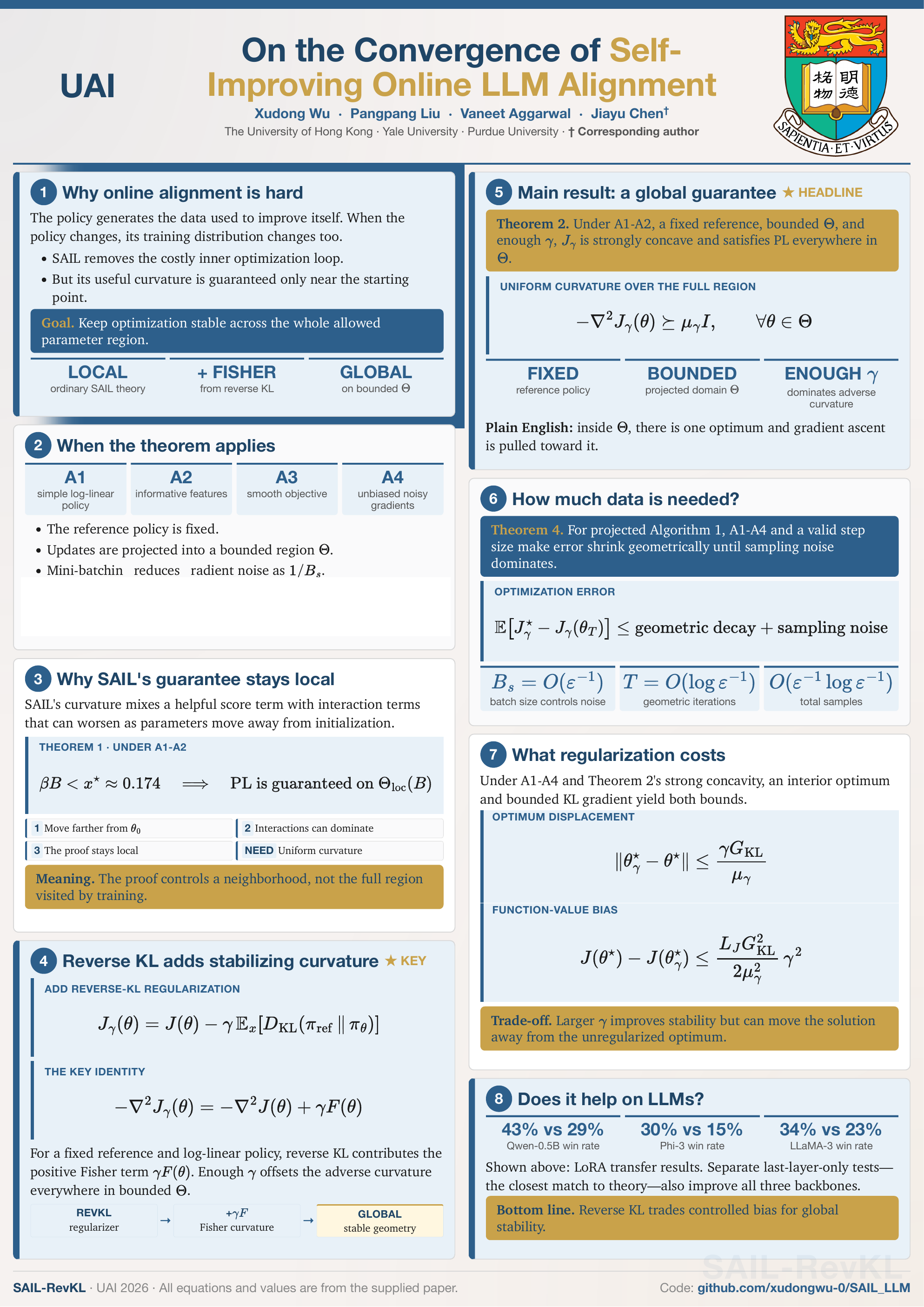
Our paper, “On the Convergence of Self-Improving Online LLM Alignment,” appeared at the 42nd Conference on Uncertainty in Artificial Intelligence (UAI 2026). It addresses a basic theoretical gap behind self-improving alignment.
Research Question
Can we establish a global convergence guarantee for online RLHF formulated as a bilevel optimization problem?
Proceedings · arXiv · Poster · MuJoCo Code · ** Code**
TL;DR
Our answer is conditional but positive. We first show that the original Self-Improving Alignment (SAIL) objective is guaranteed to have favorable curvature only near its initialization. We then introduce SAIL-RevKL, which adds
$$ \gamma\,\mathbb{E}_x!\left[ D_{\mathrm{KL}}!\left( \pi_{\mathrm{ref}}(\cdot\mid x)\,\Vert\,\pi_\theta(\cdot\mid x) \right) \right] $$
as a penalty. For a fixed reference and a log-linear policy, the Hessian of this reverse KL is the Fisher information matrix. With enough regularization, that positive curvature dominates the adverse curvature of SAIL throughout the full bounded parameter region. This yields global strong concavity and a Polyak-Lojasiewicz (PL) condition for the regularized surrogate, together with near-linear dependence on the inverse target accuracy.
Why Bilevel-Formulated Online RLHF Is Hard
Offline preference optimization trains on a fixed dataset. Online RLHF instead couples two learning problems: a reward model is fitted from preferences over responses generated by the current policy, and the policy is updated against that learned reward. This interaction is naturally formulated as a bilevel optimization problem because the solution of one level determines the objective and data distribution of the other.
SAIL uses the reward-policy equivalence to reduce this computationally expensive bilevel problem to an efficient single-level surrogate. If $\mathcal{D}_\theta$ denotes the policy-dependent response and preference distribution, that surrogate has the form
$$ J(\theta) = \mathbb{E}_{(x,y_w,y_l)\sim\mathcal{D}_\theta} !\left[ \log\sigma!\left( \beta\log\frac{\pi_\theta(y_w\mid x)}{\pi_{\mathrm{SFT}}(y_w\mid x)} - \beta\log\frac{\pi_\theta(y_l\mid x)}{\pi_{\mathrm{SFT}}(y_l\mid x)} \right) \right]. $$
This dependence matters. Standard performance-difference arguments assume that the reward or evaluation measure is independent of the policy appearing inside the advantage. That assumption no longer holds here, so convergence cannot be inherited directly from ordinary policy-gradient analysis. We instead analyze the geometry of $J$ itself.
The negative Hessian of $J$ decomposes into four terms. Some are stabilizing, while interaction terms can become unfavorable as $\theta$ moves away from the initial SFT parameters $\theta_0$. The proof must therefore control the objective’s curvature throughout the region the algorithm may visit, not only at its starting point.
Hint: why the research question is hard. In this bilevel formulation of online RLHF, the reward-learning level depends on data from the current policy, while the policy-update level depends on the learned reward. The two levels therefore evolve together, so a fixed-data convergence argument does not directly apply.
Assumptions and Scope
The global theorem is explicit about its scope. It applies to the following setting:
| Assumption | Mathematical condition | Role in the analysis |
|---|---|---|
| A1: Log-linear policy | $\pi_\theta(a\mid s)\propto\exp(\theta^\top\psi(s,a))$, with $\max_{s,a}\Vert\psi(s,a)\Vert_2\le 1$ and $\Vert\theta-\theta_0\Vert_2\le B_\theta$ | Makes the objective’s curvature analyzable on a bounded parameter set. |
| A2: Informative features | $F_\rho(\theta)\succeq\mu_F I$ uniformly over the feasible set | Ensures the Fisher curvature is positive in every parameter direction. |
| A3: Smooth objective | $J_\gamma$ is $L$-smooth | Controls the change of the gradient and permits a stable stepsize. |
| A4: Stochastic gradients | Each sample gradient is unbiased and has variance at most $\sigma_g^2$ | Makes the mini-batch noise decay as $\sigma_g^2/B_s$. |
Two construction choices are also essential. The reference policy $\pi_{\mathrm{ref}}$ is fixed during the analyzed update, and projected gradient ascent keeps every iterate inside $\Theta$, the radius-$B_\theta$ Euclidean ball centered at $\theta_0$.
Scope of the result. The word “global” below means global within this full bounded feasible set. The LoRA experiments test whether the method remains useful beyond these assumptions; the last-layer-only experiments are the closest empirical match to A1.
Core Theorem: Global Convergence of SAIL-RevKL
The original SAIL surrogate is guaranteed to have favorable geometry only near its initialization. We add a reverse-KL penalty and optimize
$$ J_\gamma(\theta) = J(\theta) - \gamma\,\mathbb{E}_x!\left[ D_{\mathrm{KL}}!\left( \pi_{\mathrm{ref}}(\cdot\mid x)\,\Vert\,\pi_\theta(\cdot\mid x) \right) \right]. $$
For a fixed reference and a log-linear policy, the reverse-KL Hessian is the Fisher information matrix, so
$$ -\nabla^2J_\gamma(\theta) = -\nabla^2J(\theta)+\gamma F(\theta). $$
Theorem (Global convergence on the feasible set)
Let $\Theta$ be the radius-$B_\theta$ Euclidean ball centered at $\theta_0$. Suppose A1-A4 hold, $\pi_{\mathrm{ref}}$ remains fixed during optimization, and projected updates keep every iterate in $\Theta$. Choose $\gamma$ sufficiently large to satisfy the explicit curvature threshold in Theorem 2 of the paper, so that the Fisher term dominates the adverse curvature of the original SAIL objective throughout $\Theta$.
Then $J_\gamma$ is $\mu$-strongly concave on all of $\Theta$ and satisfies the PL inequality
$$ \Vert\nabla J_\gamma(\theta)\Vert_2^2 \ge 2\mu\left(J_\gamma(\theta_\gamma^{\ast})-J_\gamma(\theta)\right), \qquad \theta\in\Theta, $$
where $\theta_\gamma^{\ast}=\arg\max_{\theta\in\Theta}J_\gamma(\theta)$ is the unique maximizer. Moreover, for projected mini-batch stochastic gradient ascent with a valid constant stepsize, there exist constants $q\in(0,1)$ and $C>0$ such that
$$ \mathbb{E}!\left[ J_\gamma(\theta_\gamma^{\ast})-J_\gamma(\theta_T) \right] \le q^T\left(J_\gamma(\theta_\gamma^{\ast})-J_\gamma(\theta_0)\right) + \frac{C\sigma_g^2}{B_s}. $$
Thus the optimization error decreases geometrically until it reaches the mini-batch noise floor. Taking $B_s=\widetilde{\mathcal{O}}(\varepsilon^{-1})$ and $T=\widetilde{\mathcal{O}}(\log\varepsilon^{-1})$ gives an $\varepsilon$ expected function-value gap with total sample complexity
$$ \widetilde{\mathcal{O}}!\left( \varepsilon^{-1}\log\varepsilon^{-1} \right). $$
Hint: what the theorem answers. For the SAIL reduction of bilevel-formulated online RLHF, reverse KL turns a local convergence certificate into a global, non-asymptotic guarantee over the entire bounded feasible set.
The theorem is proved in a deliberately controlled log-linear setting. We next test whether the same regularized objective is useful when training real language models.
LLM Alignment Results
The main experiments use LoRA fine-tuning and GPT-4 as an LLM judge. PKU-SafeRLHF evaluates the balance between helpfulness and harmlessness, while UltraFeedback focuses on general instruction following. Pairwise win rate is the primary comparison below; tie rate and mean GPT score difference are reported separately because they capture different aspects of the judge outcomes.
PKU-SafeRLHF, Qwen 0.5B
| Method | Pairwise win rate | Tie rate | Mean GPT score difference |
|---|---|---|---|
| DPO | 26.0% | 14.0% | -2.209 |
| SAIL | 29.0% | 0.0% | -2.004 |
| SAIL-RevKL | 43.0% | 6.0% | -0.885 |
UltraFeedback
| Backbone | Method | Pairwise win rate | Tie rate | Mean GPT score difference |
|---|---|---|---|---|
| Qwen 0.5B | DPO | 0.0% | 7.0% | -2.580 |
| Qwen 0.5B | SAIL | 1.0% | 8.0% | -2.110 |
| Qwen 0.5B | SAIL-RevKL | 3.0% | 18.0% | -1.300 |
| Phi-3 3.8B | DPO | 11.0% | 15.0% | -1.160 |
| Phi-3 3.8B | SAIL | 15.0% | 60.0% | -0.150 |
| Phi-3 3.8B | SAIL-RevKL | 30.0% | 40.0% | -0.300 |
| LLaMA-3 8B | DPO | 22.0% | 24.0% | -0.930 |
| LLaMA-3 8B | SAIL | 23.0% | 29.0% | -0.700 |
| LLaMA-3 8B | SAIL-RevKL | 34.0% | 29.0% | -0.230 |
The headline comparison is the pairwise win rate against vanilla SAIL: 43% vs. 29% on Qwen with PKU-SafeRLHF, 30% vs. 15% on Phi-3 with UltraFeedback, and 34% vs. 23% on LLaMA-3 with UltraFeedback.
A theory-aligned test
LoRA changes nonlinear features and is not a direct instantiation of the log-linear policy in A1. We therefore also freeze each backbone and train only its final linear layer on UltraFeedback U10. This isolates the regime that most closely matches the theory.
| Backbone | Method | $\gamma$ | Win rate | Lose rate | Tie rate |
|---|---|---|---|---|---|
| Qwen 0.5B | DPO | - | 1.0% | 91.0% | 8.0% |
| Qwen 0.5B | SAIL | - | 1.0% | 93.0% | 6.0% |
| Qwen 0.5B | SAIL-RevKL | $10^{-3}$ | 3.0% | 91.0% | 6.0% |
| Qwen 0.5B | SAIL-RevKL | $10^{-2}$ | 4.0% | 86.0% | 10.0% |
| Qwen 0.5B | SAIL-RevKL | $10^{-1}$ | 3.0% | 83.0% | 14.0% |
| Phi-3 3.8B | DPO | - | 13.0% | 37.0% | 50.0% |
| Phi-3 3.8B | SAIL | - | 16.0% | 40.0% | 44.0% |
| Phi-3 3.8B | SAIL-RevKL | $10^{-3}$ | 16.0% | 40.0% | 44.0% |
| Phi-3 3.8B | SAIL-RevKL | $10^{-2}$ | 21.0% | 43.0% | 36.0% |
| Phi-3 3.8B | SAIL-RevKL | $10^{-1}$ | 23.0% | 43.0% | 34.0% |
| LLaMA-3 8B | DPO | - | 0.0% | 93.0% | 7.0% |
| LLaMA-3 8B | SAIL | - | 5.0% | 69.0% | 26.0% |
| LLaMA-3 8B | SAIL-RevKL | $10^{-3}$ | 7.0% | 67.0% | 26.0% |
| LLaMA-3 8B | SAIL-RevKL | $10^{-2}$ | 7.0% | 58.0% | 35.0% |
| LLaMA-3 8B | SAIL-RevKL | $10^{-1}$ | 13.0% | 59.0% | 28.0% |
SAIL-RevKL improves the best win rate over vanilla SAIL on all three backbones. The preferred coefficient is scale-dependent: $10^{-2}$ for Qwen 0.5B and $10^{-1}$ for Phi-3 3.8B and LLaMA-3 8B. This is consistent with the theory’s curvature-bias trade-off and shows why $\gamma$ should be tuned rather than treated as a universal constant.
Hint: how to read the evidence. The LoRA results show that SAIL-RevKL improves pairwise win rates beyond the policy class covered by the theorem, but they do not prove global convergence for LoRA. Frozen-last-layer training is the closer empirical check of the log-linear regime.
Citation
@inproceedings{wu2026convergence,
  title     = {On the Convergence of Self-Improving Online {LLM} Alignment},
  author    = {Wu, Xudong and Liu, Pangpang and Aggarwal, Vaneet and Chen, Jiayu},
  booktitle = {Proceedings of the 42nd Conference on Uncertainty in Artificial Intelligence},
  pages     = {7433--7467},
  year      = {2026},
  volume    = {337},
  series    = {Proceedings of Machine Learning Research}
}
Acknowledgements
This work was supported in part by the Seed Fund for PI Research, Basic Research, from The University of Hong Kong under Project Code 2502251784.